Introduction

Recent studies have demonstrated that deep learning techniques are applicable to MRS in addressing several issues such as spectral restoration from deteriorated signals¹, ghosting artifact removal², frequency and phase correction³, and metabolite quantification⁴. However, training data size is often selected empirically or arbitrarily based on data availability and computing resources. The required training data size for adequate training of the model has not been sufficiently investigated. In this study, we evaluated the impact of training data size on the performance of deep learning in solving the spectral restoration problem as in vivo ¹H MRS data frequently suffer from low SNR and broad linewidth.

Materials and Methods

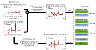
Data generation Full 3D density matrix simulations were used to generate 20 metabolite spectra including alanine, ascorbate, aspartate, creatine, gamma aminobutyric acid, glucose, glutamate, glutamine, glutathione, glycerylphos-phorylcholine, glycine, lactate, myo-inositol, N-acetylaspartate, N-acetylaspartylglutamate, phosphocholine, phosphocreatine, phosphorylethanolamine, scyllo-inositol, and taurine for a PRESS sequence at 3 T. Simulation parameters were: TE = 35 ms (TE1 = 14 ms, TE2 = 21 ms); spectral bandwidth = 4000 Hz; Shinnar-Le Roux (SLR) optimized excitation pulse (duration = 6 ms, bandwidth = 2000 Hz); and SLR optimized refocusing pulse (duration = 5 ms, bandwidth = 2000 Hz). Macromolecule signals were modeled using 13 Gaussian components.⁵ In total, 75,000 spectra were generated by randomly changing both relative metabolite concentration of individual metabolite and amplitude of individual macromolecule signals, which were considered to be the ground truth dataset. Subsequently individual spectrum was progressively degraded by broadening linewidth and adding white noise and then assigned to test dataset. SNR was measured as the ratio of signal intensity of total NAA to two times of the standard deviation of spectral noise ranging from 8 ppm to 10 ppm. Empirically, an SNR of 10 was selected as the threshold for distinguishing high SNR from low SNR.
Convolutional neural network Figure 1 shows the convolutional neural network (CNN) architecture. Each convolutional block consisted of four pairs of 1D convolutional layer and batch normalization layer. The exponential linear unit (ELU) activation function was used for the whole network. Bayesian optimization⁶ was used to find optimal network parameters including number of layers per convolutional block, kernel size, and learning rate. This process took approximately 25 hours. After assigning 70,000 spectra to training data and 5000 spectra to test data, the CNN was trained with the following number of different training subsets: 300, 500, 1000, 2500, 5000, 30,000, and 70,000 spectra. During the training phase, 20% of each training dataset was split for validation dataset. Training was performed in the complex domain so that CNN-predicted spectra can be used by spectral fitting techniques such as LCModel and jMRUI for quantifying metabolite concentrations. Thus, the input and output of the CNN had two channels for real and imaginary parts of MRS data, respectively. The CNN was trained using an Adam algorithm with a fixed learning rate of 10^-4, a batch size of 32, and 30 epochs. Mean squared error (MSE) was used as the loss function. Early stopping was applied to terminate training when the model performance ceased to improve for three epochs based on the validation dataset. The CNN was implemented and trained using the Keras library with a TensorFlow backend on a supercomputer cluster (32 GB NVIDIA Tesla V100).
CNN evaluation The CNN was trained ten times on each of the seven training sizes and then the network close to the mean MSE was assigned to be the representative one for a corresponding training size. The normalized mean squared error (NMSE) between ground truth spectra and CNN-predicted spectra was used as a metric to assess the performance of CNN. The NMSE for high SNR and low SNR was calculated from the aforementioned representative networks.

Results

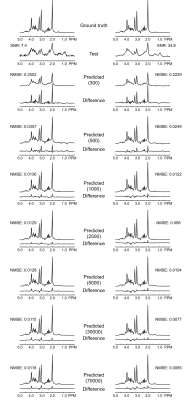
Figure 2 depicts representative simulated PRESS ¹H MRS spectra at different SNRs together with corresponding CNN-predicted spectra for different training data sizes. Visually, CNN-predicted spectra improved the most when the training sizes changed from 300 cases to 500 cases. As summarized in Table 1, the mean NMSE decreased notably from training size of 300 cases to 500 cases and showed minimal improvement at training size above 2500 cases. Likewise, the highest NMSE difference between high SNR and low SNR was observed at 300 cases (0.0379) and this difference became negligible after 2500 cases (≤ 0.0005).

Discussion

The present study demonstrated that the benefit of larger training data sizes could be marginal after reaching a threshold number of datasets in training CNN to restore degraded in vivo ¹H MRS spectra. This threshold number is expected to be dependent on the complexity of dataset. Accordingly, a reduced threshold number is predicted for less crowed data, for example, long-TE spectra, compared to the more complex dataset such as short-TE spectra used in this work. A future study is warranted to evaluate the impact of different training data sizes on accuracy and precision of metabolites quantification using CNN-predicted spectra.

Acknowledgements

No acknowledgement found.