Purpose

Magnetic resonance spectroscopy (MRS) has proven its diagnostic value for several clinical applications¹. A key factor for MRS is spectroscopic quantification. Several quantification algorithms have been proposed^2-5, while the community standard program is the commercial software LCModel^6,7. Limitations of LCModel include the fitting of the spline baseline and macromolecular background signal^8,9, and it being an expensive closed-source software not adoptable to several advanced applications. This work proposes a fitting algorithm, ProFit-v3, with adaptive baseline fitting and a new cost function. The algorithm is a further development of the previous 2D fitting software ProFit^10,11. Code will be open-source.

Theory

We define the free-induction-decay $$$\boldsymbol{\hat{y}}$$$ of an MRS spectrum ($$$\boldsymbol{\hat{Y}}$$$) as Eq. 1:$$\hat{y}=\left\{exp\left[i\frac{\pi\varphi_0}{180}-\frac{\left(\pi\,\nu_g\textbf{t}\right)^2}{4\,ln(2)}\right]\cdot\sum_k^K{c_k\boldsymbol{\beta_k}exp\left[-\pi\,\nu_{e,k}\right(TE+\textbf{t}\left)+i2\pi\omega_k\textbf{t}\right]}\right\}\otimes{}exp\left[i\frac{\pi\varphi_1}{180}\left(\boldsymbol{\delta_{ppm}}-\delta_{ref}^I\right)\right]$$where each metabolite, $$$k$$$, contributes with the concentration $$$c_k$$$, basis set $$$\boldsymbol{\beta_k}$$$, its Lorentzian line-shape parameter $$$\nu_{e,k}=\frac{1}{\pi\,T_{2,k}^*}\approx\frac{1}{\pi\,T_{2,k}}$$$ and frequency shift $$$\omega_k=\omega_{local,k}+\omega_{global}$$$. $$$\omega_{global}$$$ represents a frequency shift impacting all metabolites identically, while $$$\omega_{local,k}$$$ is individual to each metabolite. The entire spectrum is characterized by a Gaussian line-broadening factor $$$\nu_g$$$, and zeroth- and first-order phases $$$\left(\varphi_0,\varphi_1\right)$$$. The terms $$$\textbf{t}$$$ and $$$\boldsymbol{\delta_{ppm}}$$$ stand for the acquisition time and ppm vectors, $$$\delta_{ref}^I$$$ the acquisition frequency, and $$$\otimes$$$ is convolution in the time-domain. A measured spectrum ($$$\textbf{Y}$$$), however, contains both noise and a baseline (Eq. 2):$$\textbf{Y}=\hat{\textbf{Y}}+\textbf{noise}+\textbf{baseline}.$$For the spectral fitting, we define the residual $$$\textbf{R}$$$ as:$$\textbf{R}=\textbf{Y}-\hat{\textbf{Y}}-\textbf{B}\,\textbf{a}$$where $$$\textbf{B}$$$ is a vector of tensor splines modelling the baseline scaled by their corresponding spline coefficients $$$\textbf{a}$$$.
For ProFit-v3 we propose a new cost function $$$\boldsymbol{R_x}$$$ for the minimization process, composed of the frequency-domain residual $$$\boldsymbol{R}\left[\boldsymbol{\delta_{ppm}}\left(\boldsymbol{FOI}\right)\right]$$$ in the fit area of interest ($$$\textbf{FOI}$$$), the time-domain residual $$$\boldsymbol{R}\left[\boldsymbol{t}\left(1:truncPoint\right)\right]$$$ up to the signal decay point ($$$truncPoint$$$), and the weighted frequency-domain residual $$$\boldsymbol{R}\left[\boldsymbol{\delta_{ppm}}\left(\boldsymbol{FOI}\right)\right]\cdot\textbf{weights}$$$:$$\boldsymbol{R_x}=\left\{\boldsymbol{R}\left[\boldsymbol{\delta_{ppm}}\left(\boldsymbol{FOI}\right)\right]\quad\boldsymbol{R}\left[\boldsymbol{t}\left(1:truncPoint\right)\right]\quad\boldsymbol{R}\left[\boldsymbol{\delta_{ppm}}\left(\boldsymbol{FOI}\right)\right]\cdot\textbf{weights}\right\}$$The frequency-domain residual weighting is calculated from the active metabolites in the fitting iteration (Fig. 1B):$$\textbf{weights}=\sum_k^K\left\{Re\left(\boldsymbol{\beta_k}\right)>0.25\cdot{}max\left[Re\left(\boldsymbol{\beta_k}\right)\right]\right\}$$The minimization is performed on the following equation:$$\displaystyle\min_{\boldsymbol{c},\boldsymbol{a},\varphi_0,\varphi_1,\boldsymbol{\nu_e},\nu_g,\boldsymbol{\omega}}\left\|\boldsymbol{R_x}\right \|^2 + \lambda\left\|\boldsymbol{D}\,\boldsymbol{a}\right\|^2$$where $$$\lambda$$$ is the regularization parameter controlling the spline baseline flexibility and $$$\textbf{D}$$$ the second-order difference operator.
The optimal value of $$$\lambda$$$ is derived using the modified-Akaike’s information criterion ($$$mAIC$$$) proposed by Wilson². For this, the effective dimension ($$$ED$$$) is defined as:$$ED=tr\left(\boldsymbol{H}\right)=tr\left(\begin{bmatrix}\boldsymbol{B}\\\sqrt{\lambda}\boldsymbol{D}\end{bmatrix}^{-1}\begin{bmatrix}\boldsymbol{B}\\0\end{bmatrix}\right)$$and the$$$\,mAIC\,$$$as:$$mAIC=ln\left[\left\|\boldsymbol{Y}-\hat{\boldsymbol{Y}}\right\|_2^2\right]+2\,m\,ED/n$$where $$$n$$$ is the number of data points and $$$m$$$ an arbitrary value set to 15. Finally, the optimal spline baseline flexibility is found by choosing the minimum $$$mAIC\,$$$value over a series of possible$$$\,\lambda$$$; and hence also$$$\,ED\,$$$values. The optimal solution to the minimization problem of $$$\boldsymbol{R_x}$$$ is found through multiple iterations. First iterations aim to determine global parameters, while later iterations permit higher degrees of freedom for individual metabolite parameters (Fig. 1A).

Methods

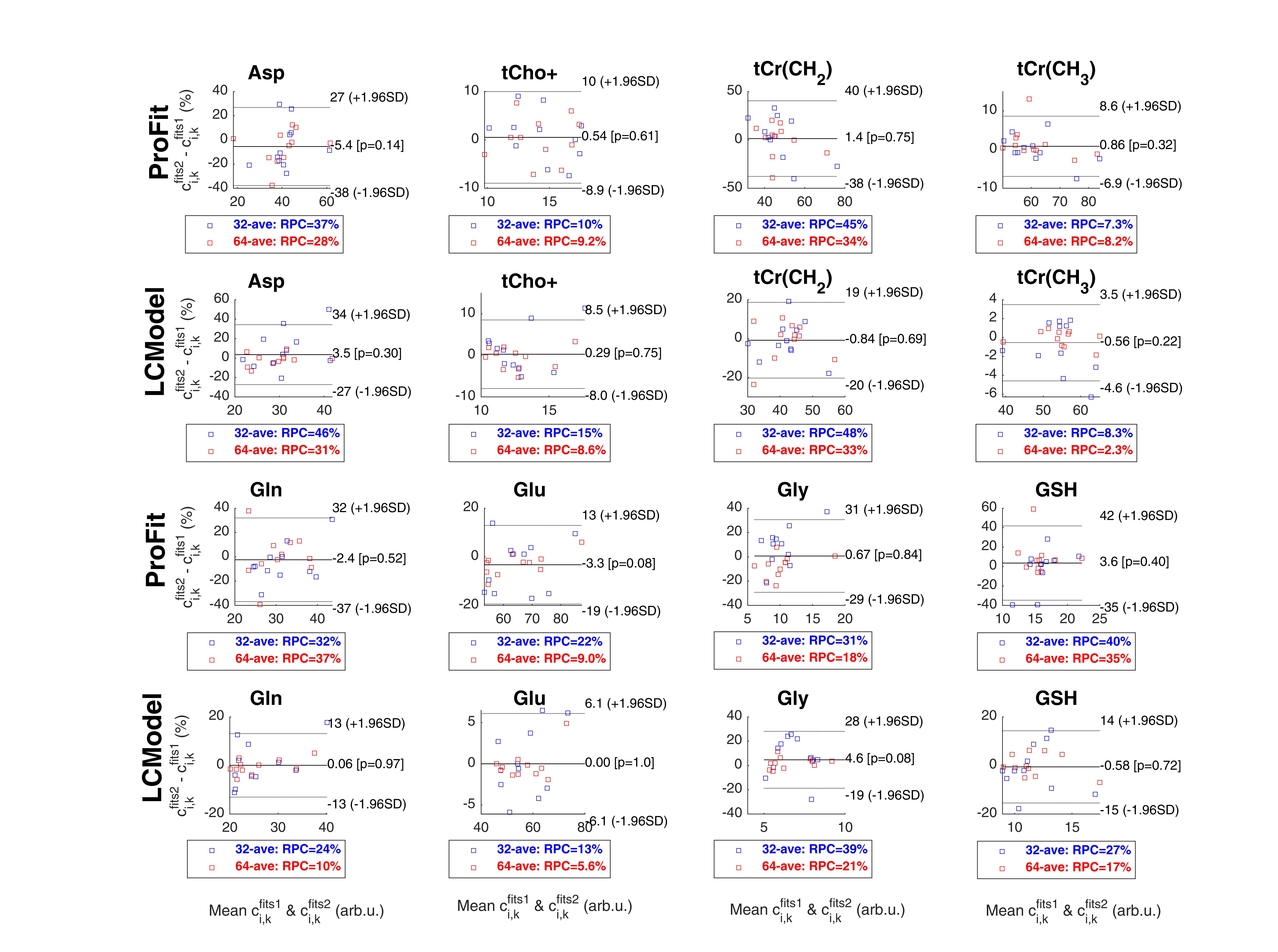
To test the accuracy and precision of ProFit-v3, in vivo quality spectra were simulated, while varying only one parameter of Eqs. 1 and 2 at a time, and keeping all others constant. Spectral baselines were created artificially to mimic typical artefacts or extracted from previous LCModel fit results of in vivo spectra (Fig. 2).
Fitting accuracy and precision were determined by comparing each fitted concentration to the simulated concentration using:$$c_{\%,k}=\frac{c_{simulated,k}-c_{fitted,k}}{c_{simulated,k}}\cdot\,100$$In vivo spectra were measured in the occipital lobe of the human brain at 9.4 T (Siemens Healthineers) with a metabolite-cycled semi-LASER sequence (TE: 24 ms, TR: 6 s, bandwidth 8 kHz, $$$\boldsymbol{\delta_{ref}}$$$ 7.0 ppm, NEX 96) in eleven healthy volunteers (27.8±1.9 years, three females). Data were preprocessed as described in Murali-Manohar et al.¹² To test in vivo reproducibility, two sub-spectra with 64 averages and two sub-spectra with 32 averages were created. The test-retest concentration results ($$$c_{i,k}^{fits1}$$$ and $$$c_{i,k}^{fits2}$$$) from the $$$i$$$ subjects for both the 32 and 64 averages sub-spectra were plotted using Bland-Altman plots¹³. Percentual concentration changes are shown via the y-axes, while reproducibility coefficients¹³ ($$$RPC$$$) are reported in the legends.

Results

A sample of the simulated baseline variations and fit results of ProFit-v3 and LCModel are shown in Fig. 2.
The accuracy and precision analysis for concentration estimates for the spectra simulated with individual parameter variations is presented in Fig. 3.
Similar fit quality is observed for the in vivo spectra fitted by ProFit-v3 and LCModel (Fig. 4).
The Bland-Altman plots of the in vivo test-retest data are shown in Fig. 5. These reveal that LCModel has on average a 2-10% higher precision than ProFit-v3 for the fitted concentrations (also depending on SNR).

Discussion

Both ProFit-v3 and LCModel fitted the spectra with the simulated baseline variations well (Fig 2). The fitted baselines show the same trends for both fitting software, and the residual is minimal. The $$$mAIC$$$ curves detected the needed baseline flexibility well and in a fully automatized manner.
The individual parameter variations in Fig. 3 show that while the ProFit-v3 fit results were slightly more accurate, the LCModel fit results are somewhat more precise. Lower concentration and coupled spin system metabolites are fitted less accurately by LCModel, whereas ProFit-v3 is less precise for these. Similarly, LCModel had a higher reproducibility for in vivo spectra; however, the ground truth for these is not known.
While LCModel is a commercial software optimized for 30 years, the fit results from the new ProFit-v3 software are very promising.

Conclusion

The newly developed open-source ProFit-v3 fitting algorithm was evaluated for both accuracy and precision with simulated and in vivo spectra. In comparison with LCModel, ProFit-v3 was slightly more accurate; however, LCModel proved to be somewhat more precise.

Acknowledgements

This project was co-sponsored by the Horizon 2020 grant / CDS-QUAMRI / 634541, the ERC Starting grant / SYNAPLAST / 679927, and the Cancer Prevention and Research Institute of Texas (CPRIT) grant / RR180056.