1839
A Deep Learning Approach to QSM Background Field Removal: Simulating Realistic Training Data Using a Reference Scan Ground Truth and Deformations1Medical Physics and Biomedical Engineering, University College London, London, United Kingdom
Synopsis
Current techniques for background field removal (BGFR), essential for quantitative susceptibility mapping, leave residual background fields and inaccuracies near air-tissue interfaces. We propose a new deep learning method aiming for robust brain BGFR: we trained a 3D U-net with realistic simulated and in-vivo data augmented with spatial deformations. The network trained on synthetic data predicts accurate local fields when tested on synthetic data, (median RMSE = 49.5%), but is less accurate when tested on in-vivo data. The network trained and tested on in-vivo data performs better, suggesting our synthetic set did not fully capture the complexity found in vivo.
Introduction
Quantitative susceptibility mapping (QSM) uses phase images to calculate the underlying tissue magnetic susceptibility and background field removal (BGFR) is a crucial step in the QSM pipeline1. The total field in the brain (Btot) is created by susceptibility sources located both inside (inducing the “local” field, Bint), and outside the brain (inducing the background field, Bext). BGFR aims to eliminate these background fields to obtain Bint from which the susceptibility is calculated. Existing BGFR techniques2 are based on assumptions (e.g. no harmonic Bint) which are often violated, leading to residual Bext and inaccuracies near air-tissue interfaces.We trained a deep learning network using realistic simulated and in-vivo data augmented using random spatial deformations, aiming to perform accurate and robust BGFR in the brain.
Methods
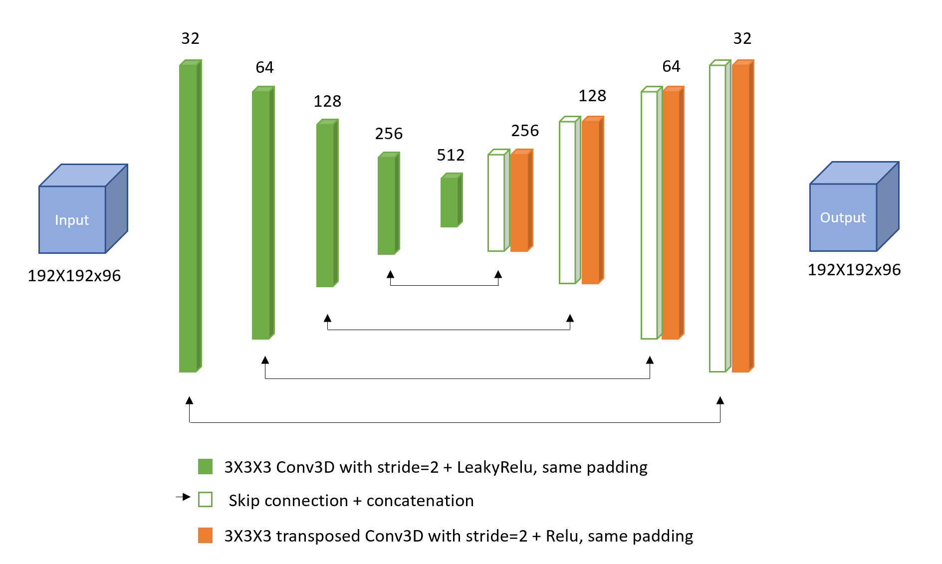
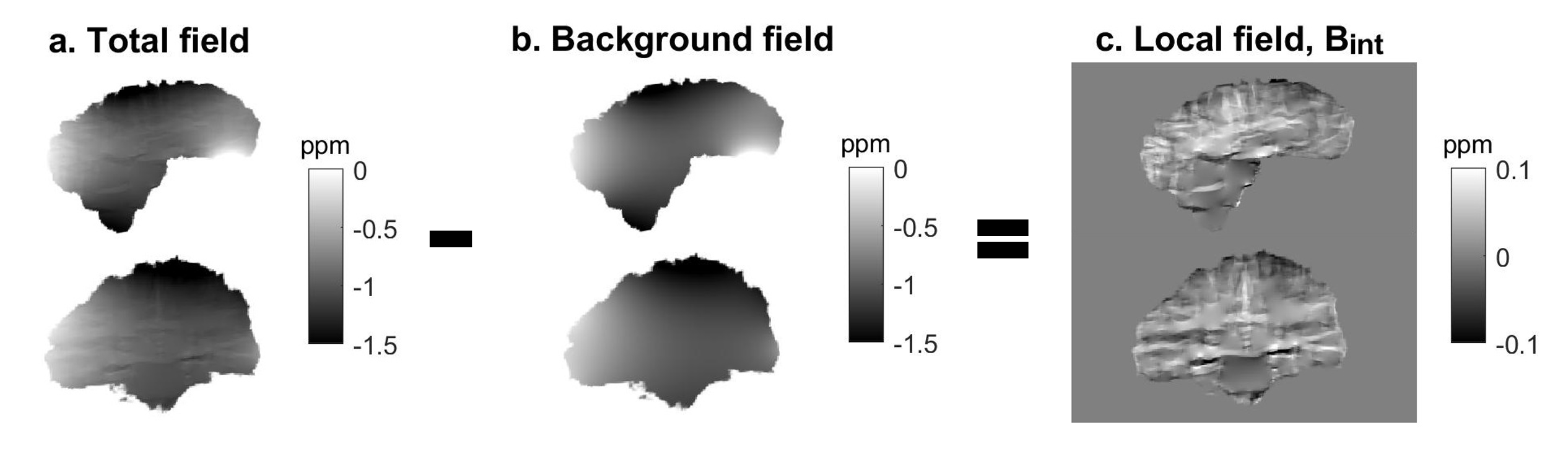
An adapted convolutional neural network (CNN), a 3D U-net created for QSM reconstruction3 (Figure 1), was trained using a synthetic dataset (Model 1) and an in-vivo dataset (Model 2).Model 1: Realistic field variations were simulated in an anthropomorphic head-and-neck phantom4. To mimic different head shapes, random spatial deformations were performed by applying B-Spline transformations with control point spacing=8 voxels and amplitude range=6 voxels and again with spacing=64 voxels, amplitude ranges=20 voxels, using a Matlab toolkit for nonrigid image registration5. Realistic susceptibility values randomly varying between ±0.2 ppm were assigned to nine different brain structures. Baseline tissue and air susceptibilities were set to -9.4 ppm and 0 ppm, respectively. Btot and Bint pairs were calculated using the simulated reference scan method4 (Figure 2): 1. Btot were computed from the susceptibility maps (all sources) using the forward model6, 2. Bext were calculated6 from maps containing only the susceptibility difference between tissue and air (outside sources) i.e. without any susceptibility structures in the brain, and 3. Bint=Btot-Bext. Noise normally distributed between ±0.02 ppm was added to the Btot input maps, while Bint ground truth maps were kept noise-free.
For training and testing, 90 and 10 pairs, respectively, of input Btot maps and target Bint maps were used. The root-mean-square errors (RMSE) between the ground truth and predicted Bint for all ten test images were calculated and the median value was used to assess model accuracy.
Model 2: In-vivo head-and-neck images were acquired at 3T in 8 healthy volunteers7 with a 3D GRE sequence, 16-channel receive coil, 1.25mm isotropic voxels, 4 echoes, TE1=ΔTE/TR=4.61/22ms, SENSE R2 and flip-angle=12°. Susceptibility maps were calculated7 using nonlinear field fitting8,9, Laplacian phase unwrapping10, BGFR with projection onto dipole fields (PDF)11, and iterative Tikhonov regularisation (α = 0.11). To increase the training sample, similar to the synthetic images, the susceptibility maps were randomly deformed5 and the susceptibility values of 13 regions of interest (ROI, automatically segmented using FSL FIRST12) were varied by adding a random constant susceptibility between ±0.2 ppm to each ROI. Here, the baseline tissue susceptibility was set to -8 ppm and a random variation between ±0.1 ppm was added to realistically augment Btot. For training, a set of 100 images was generated and downsampled by a factor of 2 to reduce computational requirements. The CNN architecture and hyperparameters (batch size=3, no. of epochs=1000) were the same as for Model 1 (Figure 1).
Models 1 and 2 were tested on Btot maps calculated (using nonlinear field fitting and Laplacian phase unwrapping) from brain images acquired at 3T4 in five healthy female volunteers using a 3D GRE sequence, 32-channel receive coil, 1mm isotropic voxels, 5 echoes, TE1/ΔTE/TR = 3/5.4/29ms, SENSE R1x2x1.5 and flip-angle=20°.
Both models' performance was compared to that of PDF.
Results
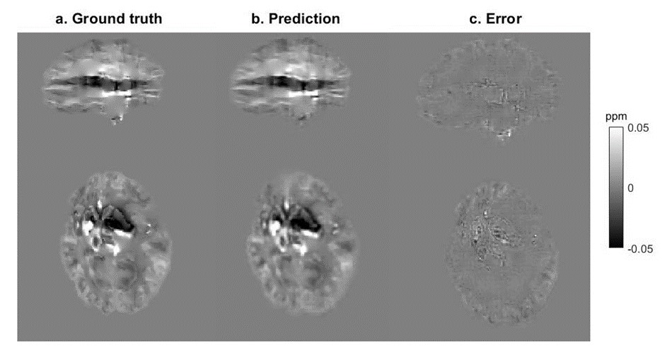
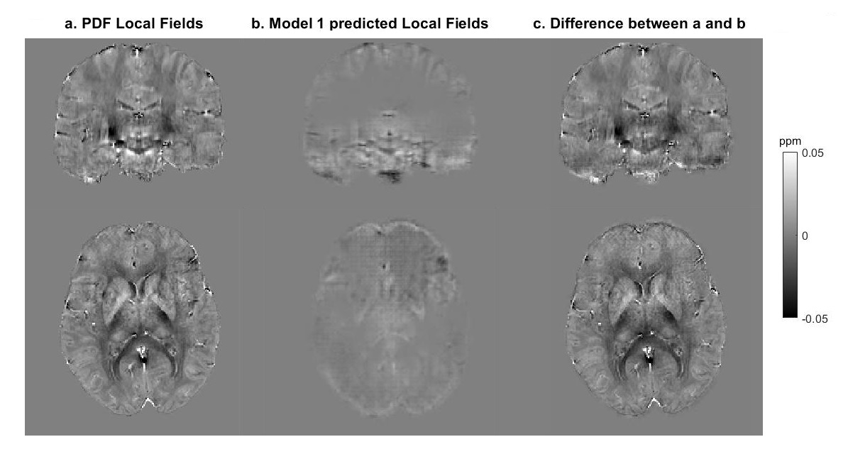
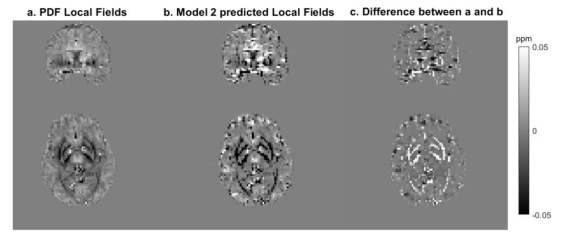
For Model 1, the median RMSE across subjects was 49.5%. Figure 3 shows an example of the ground truth and predicted Bint together with their difference. The results of testing Model 1 in vivo are presented in Figure 4. An example of the performance of Model 2 is shown in Figure 5.Discussion
When tested on synthetic data, the network trained on synthetic data, Model 1, predicts accurate Bint, close to the ground truth, with reduced artifacts near brain edges (Figure 3) compared to the results of existing techniques2. However, this network’s accuracy was much lower when tested in vivo (Figure 4). Bint were underestimated by an order of magnitude and a checkered field pattern was present probably because the synthetic training set did not fully capture the complexity of in-vivo data.Model 2, trained on in-vivo images, performed better than Model 1 when tested on in-vivo images. Figure 5 shows that Bint were still slightly underestimated compared with PDF, particularly at susceptibility interfaces/edges. We plan to use a larger training sample, consisting of both synthetic and in-vivo images with a wider range of resolutions, to minimise these differences.
Conclusion
We designed a new deep learning method for BGFR by using random spatial deformations to simulate realistic total and background fields in a numerical phantom and to augment total field maps in vivo, and using these two datasets to train a CNN. The network trained on synthetic images performs significantly better when tested on synthetic data than on in-vivo volunteer data. Training the CNN on augmented in-vivo images increased its accuracy for predicting local field maps for in-vivo images.Acknowledgements
Dr Karin Shmueli is supported by European Research Council Consolidator Grant DiSCo MRI SFN 770939.References
1. E. Haacke, S. Liu, S. Buch, W. Zheng, D. Wu and Y. Ye. Quantitative susceptibility mapping: current status and future directions. Magnetic Resonance Imaging, vol. 33, no. 1, pp. 1-25, 2015. Available: 10.1016/j.mri.2014.09.004.
2. F. Schweser, S. Robinson, L. de Rochefort, W. Li and K. Bredies. An illustrated comparison of processing methods for phase MRI and QSM: removal of background field contributions from sources outside the region of interest. NMR in Biomedicine, vol. 30, no. 4, p. e3604, 2016. Available: 10.1002/nbm.3604.
3. S. Bollmann. Deep learning QSM tutorial OHBM. Colab.research.google.com, 2018. [Online]. Available: https://colab.research.google.com/github/brainhack101/IntroDL/blob/master/notebooks/2019/Bollman/Steffen_Bollman_Deep_learning_QSM_tutorial_OHBM.ipynb. [Accessed: 13- Jan- 2020].
4. Karsa, A., Punwani, S. and Shmueli, K. The effect of low resolution and coverage on the accuracy of susceptibility mapping. Magnetic Resonance in Medicine, 81(3), pp.1833-1848, 2018.
5. Dirk-Jan Kroon. B-spline Grid, Image and Point based Registration, 2020. [Online]. Available: https://www.mathworks.com/matlabcentral/fileexchange/20057-b-spline-grid-image-and-point-based-registration), MATLAB Central File Exchange. Retrieved December 14, 2020.
6. Marques, J. and Bowtell, R. Application of a Fourier-based method for rapid calculation of field inhomogeneity due to spatial variation of magnetic susceptibility. Concepts in Magnetic Resonance Part B: Magnetic Resonance Engineering, 25B(1), pp.65-78, 2005.
7. Karsa, A., Punwani, S., & Shmueli, K. An optimized and highly repeatable MRI acquisition and processing pipeline for quantitative susceptibility mapping in the head‐and‐neck region. Magnetic Resonance in Medicine, 84(6), 3206-3222, 2020.
8. Liu T, Wisnieff C, Lou M, Chen W, Spincemaille P, Wang Y. Nonlinear formulation of the magnetic field to source relationship for robust quantitative susceptibility mapping. Magnetic Resonance in Medicine, 69(2), 467-476, 2013.
9. Cornell MRL. MEDI toolbox. [Online]. Available: http://weill.cornell.edu/mri/pages/qsm.html.
10. Biondetti E, Thomas DL, Shmueli K. Application of Laplacian-based methods to multi-echo phase data for accurate susceptibility mapping. In: Proceedings of ISMRM 24th Annual Meeting, Singapore; 2016:1547.
11. Liu, Tian, et al. A novel background field removal method for MRI using projection onto dipole fields. NMR in Biomedicine, 24(9), 1129-1136, 2011.
12. Patenaude, B., Smith, S. M., Kennedy, D. N., & Jenkinson, M. A Bayesian model of shape and appearance for subcortical brain segmentation. Neuroimage, 56(3), 907-922, 2011.
Figures