1837
Shearlet-based susceptibility map reconstruction with additional TGV-regularization
Janis Stiegeler1,2 and Sina Straub1
1Medical Physics in Radiology, German Cancer Research Center (DKFZ), Heidelberg, Germany, 2Faculty of Physics and Astronomy, University of Heidelberg, Heidelberg, Germany
1Medical Physics in Radiology, German Cancer Research Center (DKFZ), Heidelberg, Germany, 2Faculty of Physics and Astronomy, University of Heidelberg, Heidelberg, Germany
Synopsis
The 2016 Reconstruction Challenge urged the need of QSM algorithms which minimize several classical image quality measures relatively to a ground truth, but also achieve an acceptable human image perception by avoiding oversmoothing effects. A multicale shearlet system was used together with a total generalized variation (TGV) term to regularize the susceptibility-phase convolution problem. The results show that these regularizers are useful to obtain quantitative susceptibility maps which are rich in detail and simultaneously can achieve top five results in the ranking of the 2016 Reconstruction Challenge regarding all classical image quality measures used in this challenge.
INTRODUCTION
Oversmoothed susceptibility maps were a major problem of the outcome of the 2016 QSM Reconstruction Challenge (RC2016)1. The purpose of this work is to show the usefulness of a shearlet-based reconstruction supported by TGV regularization to obtain detailed susceptibility maps within a top five ranking regarding the image quality measures and algorithms used in this challenge. This work is an extension and an improvement of the algortihm presented at the ISMRM Meeting 20202.THEORY
To map the tissue magnetic susceptibility one solves a susceptibility-phase-convolution-problem: $$ \mathcal{F}(\psi) (\textbf{k}) = D(\textbf{k}) \mathcal{F}(\chi) (\textbf{k}) , \quad \textbf{k} = (k_x,k_y,k_z) \in \mathbb{R}^3, \quad (1)$$ Here $$$\mathcal{F}$$$ denotes the Fourier transform, $$$\psi$$$ the measured phase data, $$$\chi$$$ the tissue magnetic susceptibility to be determined and $$$D$$$ the dipole kernel: $$ D(\textbf{k}) := \frac{1}{3}- \frac{k_z^2}{|\textbf{k}|^2}. $$ Equation (1) is ill-posed due to $$$D(\textbf{k}) = 0$$$ at the zero cone $$$\Gamma_0$$$, $$\Gamma_0=\lbrace \textbf{k} \in \mathbb{R}^3 | k_x^2+k_y^2-2k_z^2 = 0 \rbrace.$$ Prior knowledge (e.g. sparsity under a multilevel transform $$$\Psi$$$) must be used to achieve a unique solution without artifacts. Denote by $$$\chi^*$$$ the true susceptibility, and by $$$E=\mathcal{F}^{-1}D\mathcal{F}$$$ the forward operator. Then the minimization problem $$ \underset{\chi}{min} ||W\Psi \chi||_1 + \frac{\beta}{2}||\psi-E\chi||_2^2 $$ with weights $$ W = \text{diag}(\sigma_1,...,\sigma_N) \quad \text{and} \quad \sigma_i = \begin{cases} \frac{1}{|\Psi \chi_i^*|}, \quad & \Psi x_i \neq 0, \\ \infty, \quad & otherwise,\end{cases} $$ will find sparser solutions than the unweighted minimization problem3. Instead of the true solution, one considers a sequence of weights $$ \sigma_i^k = \frac{1}{|(\Psi \chi^k)_i|+ \epsilon}, $$ where $$$\epsilon > 0$$$ is small and $$$(\chi^k)_k \subset \mathbb{R}^N$$$ are approximations to the true susceptibility $$$\chi^*$$$, given by $$\chi^k = \underset{\chi}{\text{argmin}}||W^{k-1}\Psi \chi||_1 + \frac{\beta}{2}||y-E\chi||_2^2. $$ The coefficients of a multiscale transform decrease with higher scales. To avoid erroneous zero coefficients4,5, the weighting matrix $$$W$$$ is therefore given scalewise. $$ W^j_{k+1}d^j = diag\left(\frac{\lambda_j^{k+1}}{|(\Psi x_{k+1})_j|+ \epsilon}\right)d^j, $$ where $$$\Psi x = \left(\Psi_j x\right)_{j=0,...,J} = \left(\langle \Psi_{j,l},x \rangle \right)_{j = 0,...,J,l=1,...,N_j},$$$ divides the shearlet coefficients into $$$J$$$ scales and $$$\lambda_j^{k+1} = \underset{l}{max} \left(\langle \Psi_{j,l},x_{k+1} \rangle \right)_l $$$ denotes the maximum of the shearlet coefficients of $$$x_{k+1}$$$ belonging to scale $$$j$$$.METHODS
The RC2016 provided local phase data, two different ground truths and four error metrics1. To compute the image quality measures, $$$\chi_{33}$$$ from the STI solution was used as ground truth. For a further comparison a susceptibility map was reconstructed with the STAR-QSM algorithm6.The proposed algorithm consists of three steps. In Step 1 a susceptibility map $$$\chi_{well}$$$ from the data in the well-conditioned region $$$(|D| > 0.2)$$$ is calculated by an LSQR method7. The second step includes $$$\chi_{well}$$$ as an additional data-fit term7 in the following problem: $$\underset{\chi}{min} ||\Psi \chi||_1 + \alpha TGV^2(\chi) + \beta_1 ||E\chi-\psi||_2^2 + + \beta_2 ||M\chi-\chi_{well}||_2^2 \quad (2)$$ where $$$M = \mathcal{F}^{-1}R\mathcal{F}$$$ is a linear operator including the binary mask $$$R$$$ which defines the well-conditioned region and $$$\Psi$$$ is the shearlet transform8. Finally, as step 3, an additional nonlinear data fit around the solution $$$\chi$$$ of Step 2 is done : $$\underset{\tilde{\chi}}{\text{min}}||\cos(y)-\cos(E(\tilde{\chi}))||_2^2 + ||\sin(y)-\sin(E(\tilde{\chi}))||_2^2 + ||\tilde{\chi}-\chi||_2^2 \quad (3).$$ Newton's method is applied to solve Equation (3). The method of alternating direction of multipliers (ADMM) is applied in step 2 by introducing auxillary variables $$$w,d,t,b^w,b^d,b^t$$$ and three new parameters $$$\mu = (\mu_1,\mu_2,\mu_3) > 0$$$: $$ \begin{split} \chi_{k+1} &= \underset{\chi}{arg min} \:\frac{\beta_1}{2} ||E\chi-\psi||_2^2 + \frac{\beta_2}{2} || \chi_{well}- Mx||_2^2 + \frac{\mu_1}{2} ||w_k - \Psi \chi – b^w_k||_2^2 + \frac{\mu_2}{2} ||d_k – (\nabla^f \chi – v) – b^d_k||_2^ +\frac{\mu_3}{2} ||t_k -\zeta^bv – b^t_k||_2^2 2 \quad (4) \\ w_{k+1} + &= \underset{d}{arg min} \: ||w||_1 + \frac{\mu_1}{2} ||w - \Psi \chi_{k+1} – b^w_k||_2^2 \quad (5) \\ d_{k+1} + &= \underset{d}{arg min} \: ||d||_1 + \frac{\mu_2}{2} ||d – (\nabla^f \chi_{k+1} – v_{k+1}) – b^d_k) – b^d_k||_2^2 \quad (6) \\ t_{k+1} + &= \underset{t}{arg min} \: ||t||_1 + \frac{\mu_3}{2} ||t – \zeta^bv_{k+1} – b^t_k ||_2^2 \quad (7) \\ b^w_{k+1} &= b^w_k + \Psi \chi_{k+1} - w_{k+1} \\ b^d_{k+1} &= b^d_k + (\nabla^f \chi_{k+1} - v_{k+1} )- d_{k+1} \\ b^t_{k+1} &= b^t_k + \zeta v_{k+1} - t_{k+1}, \end{split}. $$ The $$$\chi$$$-update is solved by diagonalization, setting the gradient of Equation (4) to zero. The solution of Equation (5) provides the shearlet coefficients. The iterative reweighting can be directly incorperated into this subproblem by replacing Equation (5) by $$ w_{k+1} = \underset{w}{arg min} \: ||W_{k+1}w||_1 + \frac{\mu}{2} ||w - \Psi \chi_{k+1} – b^w_k||_2^2 \quad (8)$$ Equation (8) is explicitly solved by shrinking: $$ d_{k+1} = \text{shrink}\left(\Psi \chi_{k+1} + b^w_k, \frac{1}{\mu}W \right),$$ where the shrinkage function $$\text{shrink}(u,\omega) = \begin{cases} max\left(||u||-\omega,0\right)\frac{u}{||u||}, \quad &u\neq 0\\ 0,\quad \quad &u = 0 \end{cases}$$ is applied element-wise. Equation (6) and (7) are solved analogously3. For this work the parameters were chosen to minimize the quality measures but not to oversmooth the resulting susceptibility map.RESULTS & DISCUSSION
The achieved image quality measures are shown in Table 1, for the proposed algorithm (PA) and for STAR-QSM. The PA achieves entirely a top five, even two first rankings (SSIM, ROI-Error).In Figure 2, the susceptibility maps for the PA and STAR-QSM are shown together with the ground truth.
The purpose of this work is to show that beside a high ranking regarding the image quality measures a detailed susceptibility map can be reconstructed using the benefits of shearlets and TGV.
Acknowledgements
This work was supported by a grant from Deutsche Forschungsgemeinschaft (Grant number: DFG STR 1480/2-1). The use of the data from the 2016 Reconstruction Challenge is kindly acknowledged. The use of code for the shearlet reweighing provided by Dr. Jackie Ma is kindly acknowledged as well as the use of the code for the shearlet transform from ShearLab3D.References
- Langkammer C. et al., Quantitative Susceptibility Mapping: Report from the 2016 Reconstruction Challenge. Magnetic Resonance in Medicine 2017; 00:00-00.
- J. Stiegeler and S. Straub, Shearlet-based susceptibility map reconstruction with iterative reweighting and nonlinear data fitting, ISMRM & SMRT Virtual Conference & Exhibition, 08-14 August 2020.
- Candès E. J. et al., Enhancing sparsity by reweighted $$$l_1$$$ minimization. J. Fourier Anal. Appl., vpl. 14, no. 5-6, pp. 877-905, 2008
- Ma J. and März M., A multilevel based reweighting algorithm with joint regularizers for sparse recovery. arXiv:1604.06941 [math.OC], 2017.
- Ma J. et al.,Shearlet-based compressed sensing for fast 3D cardiac MR imaging using iterative reweighting. Physics in Medicine and Biology (2018). 63. 235004. 10.1088/1361-6560/aaea04.
- Wei HJ, Dibb R, Zhou Y, Sun YW, Xu JR, Wang N, Liu CL. Streaking artifact reduction for quantitative susceptibility mapping of sources with large dynamic range. Nmr in Biomedicine. 2015;28(10):1294-303. doi: 10.1002/nbm.3383. PubMed PMID: WOS:000363468300012.
- Kames C. et al., Rapid two-step dipole inversion for susceptibility mapping with sparsity priors. NeuroImage Volume 167, 15 February 2018, Pages 276-283.
- G. Kutyniok, W.-Q. Lim, R. Reisenhofer, ShearLab 3D: Faithful Digital Shearlet Transforms Based on Compactly Supported Shearlets. ACM Trans. Math. Software 42 (2016), Article No.: 5. www.shearlab.org.
Figures
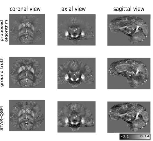
Figure 1: In the first row the susceptibility map obtained by the proposed algorithm is shown.The second row shows the ground truth and in the third row a susceptibility map calculated by STAR-QSM is shown.
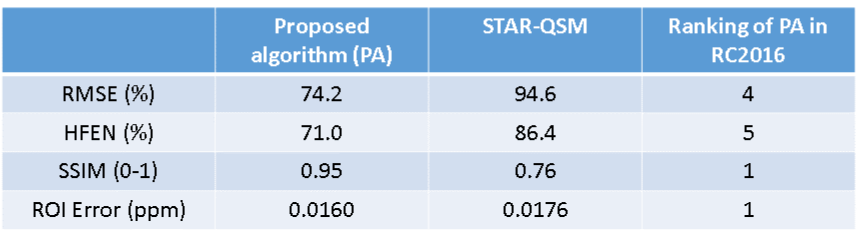
Table 1: The values for the image quality measures achieved by the susceptibility maps obtained by the proposed algorithm and by STAR-QSM are shown in the first and second column. The third column shows the achieved ranking compared to all algorithms testes in the 2016 QSM challenge. RMSE is the root mean squared error. HFEN is the high-frequeny error norm. SSIM is the structural similarity index. The ROI error is the absolute value of the mean error in selected anatomical structures as in the 2016 QSM challenge.