1832

Dipole inversion by recurrent inference for quantitative susceptibility mapping

Samy Abo Seada¹, Emanoel Ribeiro Sabidussi¹, Sebastian Weingärtner², Dirk H. J. Poot¹, and Juan Antonio Hernandez-Tamames¹
¹Department of Radiology and Nuclear Medicine, Erasmus MC, Rotterdam, Netherlands, ²Department of Imaging Physics, TU Delft, Delft, Netherlands

Synopsis

QSM dipole inversion remains a challenge and recent machine learning approaches have not incorporated the known forward model directly. We propose using recurrent inference machines (RIM), a type of unrolled optimization technique, which are proposed for solving iterative inverse problems specifically. RIMs enable incorporating the forward dipole convolution directly in the learning process. Simulated data was used for training. The QSM reconstruction was tested on simulated data and healthy subject data acquired at 3T.

Introduction and background

Quantitative susceptibility mapping (QSM) is a promising quantitative MR technique sensitive to tissue susceptibilities. QSM can be used to depict iron deposits, small veins, calcium and myelin^1,2. The dipole inversion step unfolds the biophysical effect of tissue susceptibility on the measured MR signal and is a challenge in the post-processing pipeline.

The forward effect, under certain assumptions, of tissue susceptibility $$$\chi(r)$$$ to field shift $$$\delta f(r)$$$ can be written as a spatial convolution $$$\delta f=\chi\ast A$$$ or a Fourier multiplication^1,3
$$\delta f(\overrightarrow{r})=\int_{r_d} \chi(\overrightarrow{r}')\frac{3cos^2(\theta )-1}{4\pi |\overrightarrow{r}'-\overrightarrow{r}|}d^3r'=iFT\big( FT(\chi(\overrightarrow{r}))\times (\frac{1}{3}-\frac{k_z}{k^2})\big) \quad[1]$$
where $$$A$$$ is the dipole kernel, $$$\overrightarrow{r}$$$ the spatial location vector, $$$\theta$$$ denotes the angle between field $$$B_0$$$ and $$$|\overrightarrow{r}’-\overrightarrow{r}|$$$, $$$r_d$$$ the spatial domain sufficiently distant from $$$r$$$, (i)FT denotes an (inverse) 3D Fourier operation, and $$$\overrightarrow{k}$$$ is the frequency vector. The dipole kernel $$$A$$$ has zero-values in both spatial and frequency domains and consequently a direct inversion from $$$\delta f $$$ to $$$\chi$$$ is infeasible.

Conventional techniques use modified kernels with near zero-values⁴ or iterative regularized reconstruction techniques^5,6 while recent machine-learning approaches use 3D U-NETs^7–10 or variational regularisers¹¹. Recently inverse problem solving recurrent architectures^12–14, and specifically Recurrent Inference Machines (RIM) have been developed^15,16. RIMs perform inversion through a fixed number of inferences, and could aid machine interpretability¹⁷.

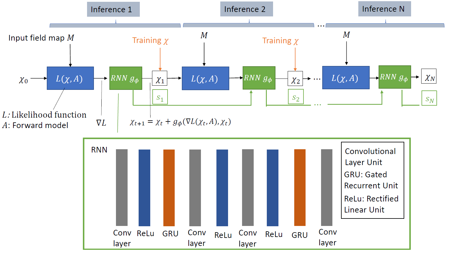
RIMs use the forward model (equation 1) and during training learn an implicit prior on the model parameters (Figure 1). The parameters at inference step $$$t$$$ are updated as $$\chi_{t+1}=\chi_t+g_{\phi}(\nabla L(\chi_t,A),\chi_t)\quad[2]$$ where the likelihood function $$$L(\chi_t,A)=\sum_{\overrightarrow{r}}(\chi_t \ast A - M)^2$$$ evaluates consistency with the input field map $$$M$$$ and $$$g_{\phi}$$$ is a Recurrent Neural Network (RNN) with the learned parameters $$$\phi$$$. The RIM is trained as
$$ \phi = \arg \min_{\phi} E_{\phi^{GT},M}\sum_t |\chi_t-\chi^{GT}|^2\quad[3]$$ where $$$\chi^{GT}$$$ denotes the ground truth susceptibility.

We developed a RIM for the purpose of dipole inversion and compare it against MEDI⁵.

Methods

The RIM was implemented in PyTorch with 6 inference steps using identical RNNs (kernel size 3, padding to preserve image size at each layer, 3D convolution stride 1). Training (batch size =10, ADAM optimizer, learning rate 1e-5) used 10’000 cubic samples of size 32 which served as ground truth susceptibility $$$\chi^{GT}$$$. These contained 60 randomly placed rectangles (p=2/3) and spheres (p=1/3) with random sizes and specific susceptibilities drawn from a normal distribution ($$$\mu$$$=0,$$$\sigma$$$=1), similar to DeepQSM⁷. Input fields $$$M$$$ were created using equation 1 without added noise. Training with 50 epochs took 15 hours on an NVIDIA RTX 2080 Ti. No validation was used. Testing was done using 1000 new samples created akin to training. For comparison MEDI⁵ reconstructions were made ($$$\lambda$$$=250).

In-vivo data was collected from a healthy volunteer using a 3T GE Discovery MR750 with an 8 channel brain coil. A 3D multi-echo gradient-echo sequence ($$$TE_1$$$=13ms,$$$\Delta TE$$$=3.3ms, $$$TE_{16}$$$=65.8ms)¹⁸ with 1mm isotropic resolution, covering from brain-stem to above deep gray nuclei. The last 3 echoes were discarded after visual inspection. Coil images were combined using estimated sensitivities^19,20. BET²¹ was used for masking, while frequency fields and phase unwrapped images were created using the MEDI toolbox^22–24. Projection onto Dipole Fields (PDF) was used to remove background fields²⁵. The relative difference fields (RDF) acted as the input field maps $$$M$$$ for both MEDI ($$$\lambda$$$=400, spherical radius 6.5) and RIM.

Results

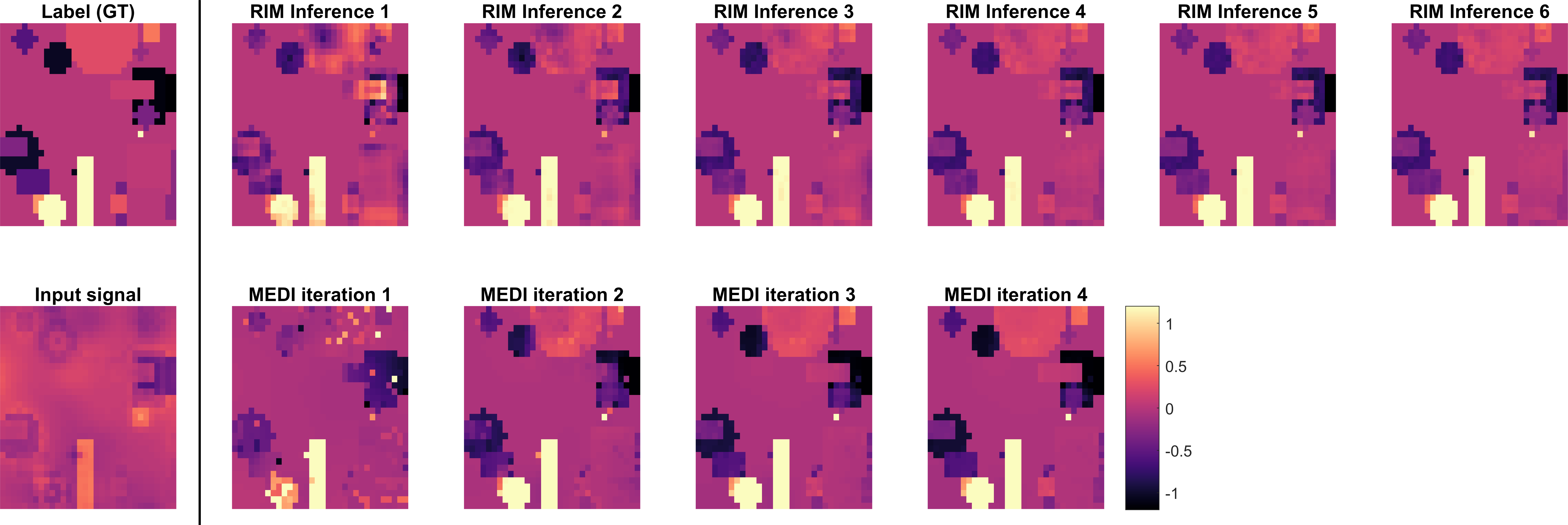
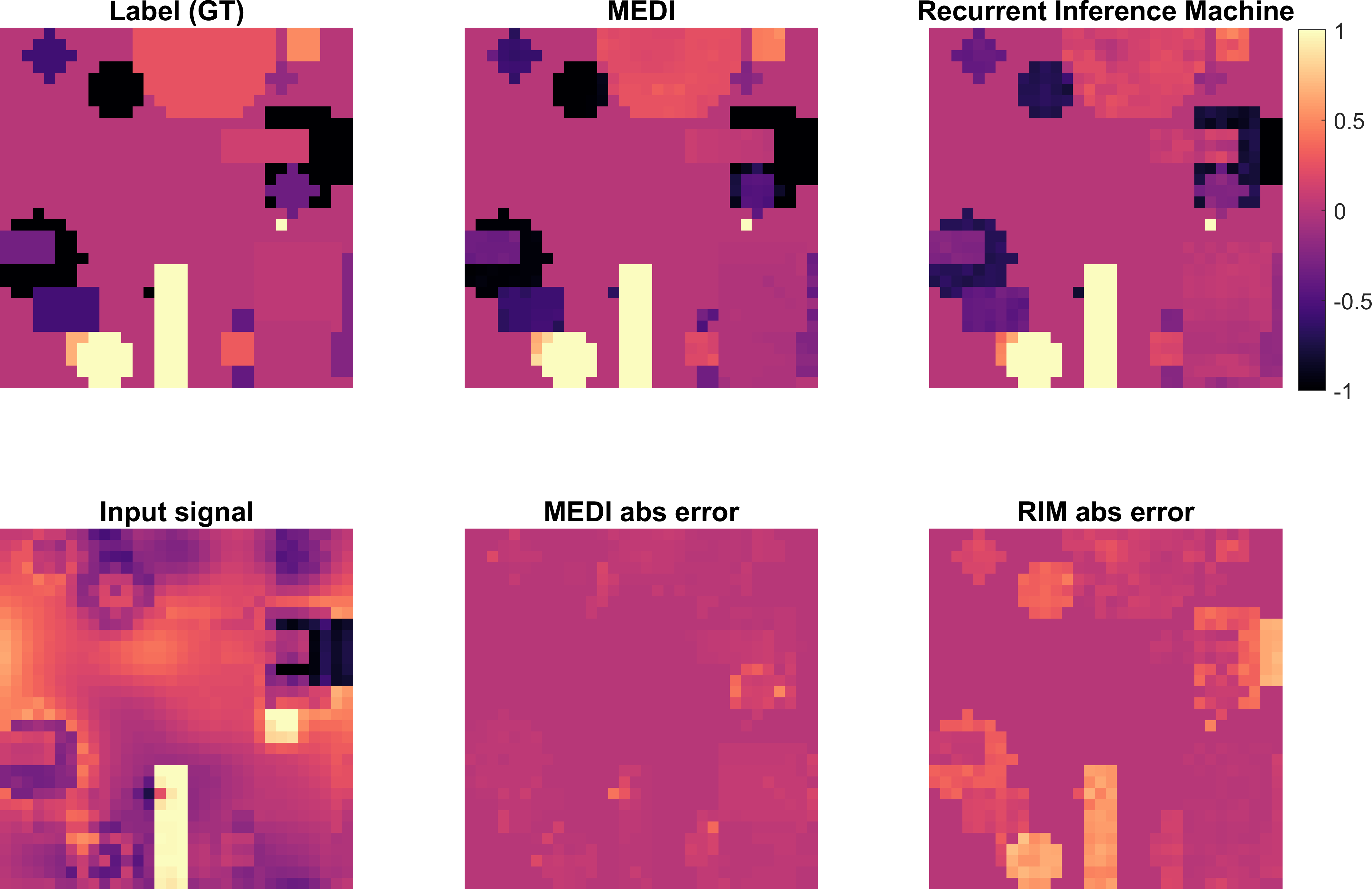
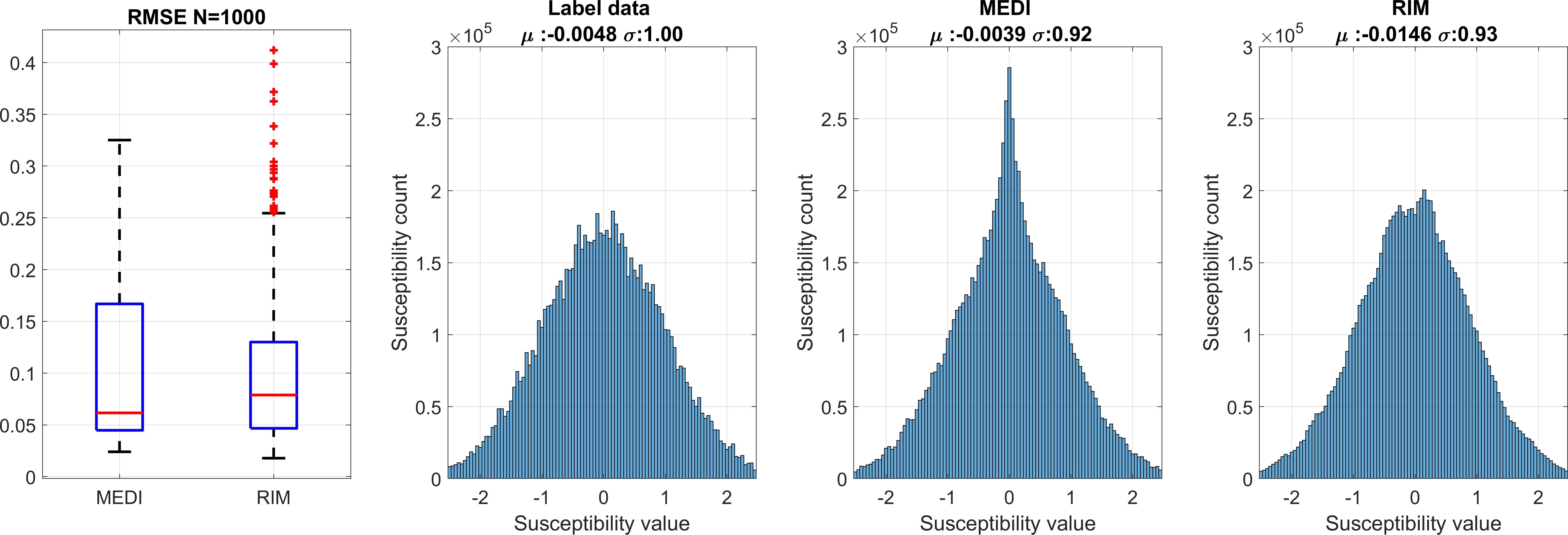
Figure 2 shows the iterative behaviour of RIM and MEDI for a testing example. Figure 3 shows simulation results between MEDI and RIM. Both approaches correctly identified shapes within the sample, however RIM over and underestimated some shapes leading to larger errors.

Quantitative analysis of the simulation data (Figure 4) shows that median RMSE was 28% higher for RIM results than for MEDI. Histograms show that MEDI has less bias than the RIM, however the RIM distribution matches more closely to the original data.

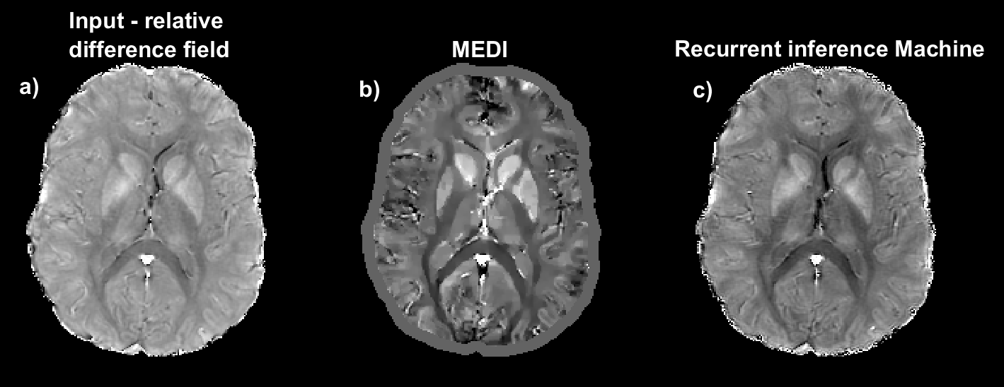
Figure 5 shows an in-vivo comparison of the input data (RDF) and the reconstructions from MEDI and RIM. MEDI successfully reconstructed high contrast in deep gray nuclei, known to have high iron content. The RIM approached darkening of myelinated regions, yet seems closer to the initial input data.

Discussion

The RIM is proposed as an alternative to 3D U-NETS for the dipole inversion problem, as they are designed to solve inverse problems based on explicit forward models. Their recurrent behaviour (Figure 2) allow for interpretability. RIM performed well on the simulation data yet was outperformed by MEDI, possibly due to estimation bias. RIM also did not perform as well as MEDI on in-vivo data. Causes could be insufficient training or unmatched training data. Future work will investigate both possibilities further, using real or simulated brain data.

The choice of network architecture defines inversion behaviour, thus, including prior knowledge. The effect of the number of inference steps remains to be investigated, as is a comparison with other machine learning approaches^7-11.

Conclusion

Recurrent Inference Machines (RIM) were shown to learn the dipole inversion problem from simulation data.

Acknowledgements

This project was funded by Convergence for healthy and technology.

S.W. acknowledges funding from the 4TU Precision Medicine program.

References

1. Schweser F, Deistung A, Reichenbach JR. Foundations of MRI phase imaging and processing for Quantitative Susceptibility Mapping (QSM). Z. Med. Phys. 2016;26:6–34 doi: 10.1016/j.zemedi.2015.10.002.

2. Reichenbach JR, Schweser F, Serres B, Deistung A. Quantitative Susceptibility Mapping: Concepts and Applications. Clin. Neuroradiol. 2015;25:225–230 doi: 10.1007/s00062-015-0432-9.

3. de Rochefort L, Liu T, Kressler B, et al. Quantitative susceptibility map reconstruction from MR phase data using bayesian regularization: Validation and application to brain imaging. Magn. Reson. Med. 2010;63:194–206 doi: 10.1002/mrm.22187.

4. Shmueli K, de Zwart JA, van Gelderen P, Li T-Q, Dodd SJ, Duyn JH. Magnetic susceptibility mapping of brain tissue in vivo using MRI phase data. Magn. Reson. Med. 2009;62:1510–1522 doi: 10.1002/mrm.22135.

5. Liu J, Liu T, De Rochefort L, et al. Morphology enabled dipole inversion for quantitative susceptibility mapping using structural consistency between the magnitude image and the susceptibility map. Neuroimage 2012;59:2560–2568 doi: 10.1016/j.neuroimage.2011.08.082.

6. Li W, Wang N, Yu F, et al. A method for estimating and removing streaking artifacts in quantitative susceptibility mapping. Neuroimage 2015;108:111–122 doi: 10.1016/j.neuroimage.2014.12.043.

7. Bollmann S, Rasmussen KGB, Kristensen M, et al. DeepQSM - using deep learning to solve the dipole inversion for quantitative susceptibility mapping. Neuroimage 2019;195:373–383 doi: 10.1016/j.neuroimage.2019.03.060.

8. Yoon J, Gong E, Chatnuntawech I, et al. Quantitative susceptibility mapping using deep neural network: QSMnet. Neuroimage 2018;179:199–206 doi: 10.1016/j.neuroimage.2018.06.030.

9. Chen Y, Jakary A, Avadiappan S, Hess CP, Lupo JM. QSMGAN: Improved Quantitative Susceptibility Mapping using 3D Generative Adversarial Networks with increased receptive field. Neuroimage 2020;207:116389 doi: 10.1016/j.neuroimage.2019.116389.

10. Gao Y, Zhu X, Moffat BA, et al. xQSM: Quantitative Susceptibility Mapping with Octave Convolutional and Noise Regularized Neural Networks. 2020:1–9.

11. Polak D, Chatnuntawech I, Yoon J, et al. Nonlinear dipole inversion (NDI) enables robust quantitative susceptibility mapping (QSM). NMR Biomed. 2020;33:1–13 doi: 10.1002/nbm.4271.

12. Diamond S, Sitzmann V, Heide F, Wetzstein G. Unrolled Optimization with Deep Priors. arXiv 2017:1–11.

13. Hosseini SAH, Yaman B, Moeller S, Hong M, Akçakaya M. Dense Recurrent Neural Networks for Accelerated MRI: History-Cognizant Unrolling of Optimization Algorithms. IEEE J. Sel. Top. Signal Process. 2019;14:1280–1291 doi: 10.1109/JSTSP.2020.3003170.

14. Knoll F, Hammernik K, Kobler E, Pock T, Recht MP, Sodickson DK. Assessment of the generalization of learned image reconstruction and the potential for transfer learning. Magn. Reson. Med. 2019;81:116–128 doi: 10.1002/mrm.27355.

15. Putzky P, Welling M. Recurrent Inference Machines for Solving Inverse Problems. 2017.

16. Lønning K, Putzky P, Sonke J-J, Reneman L, Caan MWA, Welling M. Recurrent inference machines for reconstructing heterogeneous MRI data. Med. Image Anal. 2019;53:64–78 doi: 10.1016/j.media.2019.01.005.

17. Monga V, Li Y, Eldar YC. Algorithm Unrolling: Interpretable, Efficient Deep Learning for Signal and Image Processing. arXiv 2019.

18. Mazzucchi S, Frosini D, Costagli M, et al. Quantitative susceptibility mapping in atypical Parkinsonisms. NeuroImage Clin. 2019;24:101999 doi: 10.1016/j.nicl.2019.101999.

19. Walsh DO, Gmitro AF, Marcellin MW. Adaptive reconstruction of phased array MR imagery. Magn. Reson. Med. 2000;43:682–690 doi: 10.1002/(SICI)1522-2594(200005)43:5<682::AID-MRM10>3.0.CO;2-G.

20. Sun H. QSM software. https://github.com/sunhongfu/QSM.

21. Smith SM. Fast robust automated brain extraction. Hum. Brain Mapp. 2002;17:143–155 doi: 10.1002/hbm.10062.

22. Kressler B, de Rochefort L, Tian Liu, Spincemaille P, Quan Jiang, Yi Wang. Nonlinear Regularization for Per Voxel Estimation of Magnetic Susceptibility Distributions From MRI Field Maps. IEEE Trans. Med. Imaging 2010;29:273–281 doi: 10.1109/TMI.2009.2023787.

23. de Rochefort L, Brown R, Prince MR, Wang Y. Quantitative MR susceptibility mapping using piece-wise constant regularized inversion of the magnetic field. Magn. Reson. Med. 2008;60:1003–1009 doi: 10.1002/mrm.21710.

24. Liu T, Wisnieff C, Lou M, Chen W, Spincemaille P, Wang Y. Nonlinear formulation of the magnetic field to source relationship for robust quantitative susceptibility mapping. Magn. Reson. Med. 2013;69:467–476 doi: 10.1002/mrm.24272.

25. Liu T, Khalidov I, de Rochefort L, et al. A novel background field removal method for MRI using projection onto dipole fields (PDF). NMR Biomed. 2011;24:1129–1136 doi: 10.1002/nbm.1670.

Figures

Figure 1 - Recurrent inference machine (RIM), in an unrolled fashion. RIM learns solving an inverse problem given a forward model A. Susceptibility is estimated from MR signal using fixed N inference steps. Each step contains likelihood estimation (blue) followed by an RNN (green) which outputs an update term $$$g_{\phi}$$$, learned through network training. A prior distribution is not specified, but the gradient of a prior probability is learned through hidden states s. The RNN is detailed in the bottom panel with 3D convolutional layers, which train $$$g_\phi$$$ over time.

Figure 2 - The RIM inference process for an axial example drawn from the testing data, along with each estimate from the iterative MEDI procedure. The label (ground truth) and input signal are shown in the left-most column. In both techniques the shapes become clearly defined with increasing iterations, as expected. The initial inference from RIM resolve many shapes, but with an incorrect susceptibility range (e.g. sphere, middle-left) which does not get corrected over inferences. MEDI on the other hand converges closer to the label data.

Figure 3 - Simulated results using squares and spheres, which served as training data for the recurrent inference machine (RIM). Top rows shows (left to right) the ground truth, MEDI and RIM results. Qualitatively MEDI and RIM reconstruct similarly, however RIM reconstructions incorrectly estimated variations within shapes (top sphere). Bottom row shows the input signal, and the absolute error between each technique and the label image. Apart from generic errors, RIM under and overestimates the susceptibility value of entire shapes.

Figure 4 - Quantitative analysis of simulation results. Across 1000 samples RIM had a 28.0% higher median RMSE than MEDI. Histogram plots are shown for label data, MEDI and RIM reconstructions. MEDI has noticeably less bias than the RIM (-0.0039 vs -0.0146), however the RIM distribution matches more closely to the original data.

Figure 5 - In-vivo results acquired at 3T showing the a) preprocessed input image, used as a starting point for both b) MEDI and the c) Recurrent Inference Machine (RIM). The MEDI results shows high contrast in the deep nuclei regions associated with higher iron content. However, the image gets smoothed by the spherical filter. The RIM result has some element from the MEDI image such as dark contrast in the myelin regions, yet remains similar to the input image to a large extent. Possibly, the network did not complete training, or the training data was unsuited to this problem.

Proc. Intl. Soc. Mag. Reson. Med. 29 (2021)

1832