Introduction

Individual iron oxide nanoparticle labelled immune cells can be visualized with a dynamic MRI image series. Time-lapse MRI can provide insights in the studies of inflammatory diseases and metastasis of cancer. Current study, however, cannot detect cells traveling faster than 1µm/s due to temporal blurring¹. The temporal resolution can be improved by undersampling k-space. However, the optimal acceleration factor cannot be easily determined prior to experiments. Strategies have been proposed for non-Cartesian flexible retrospective undersampling². These methods require significant modification on the pulse sequence and may not be readily applicable for most users. We propose a Cartesian sampling scheme where undersampling ratio and temporal resolution can be chosen retrospectively.

Methods

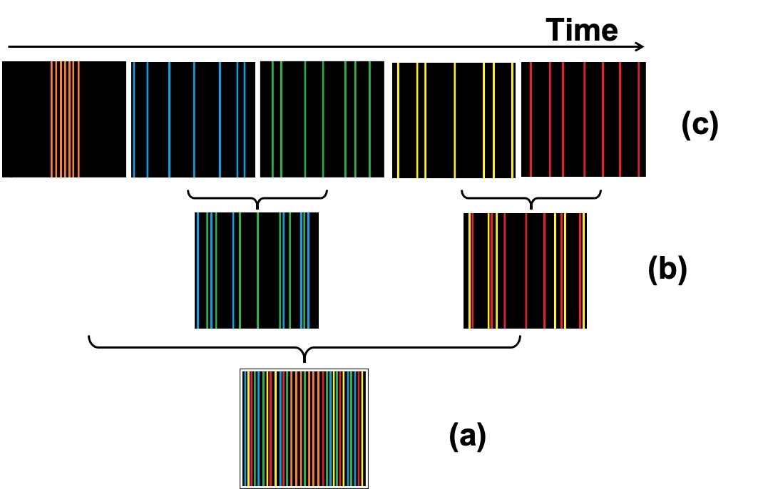
The 2D Cartesian scheme is illustrated in Fig. 1. The central lines of k-space are first acquired. The high frequency lines are sampled in a special sequence that has relatively uniform coverage, with incoherent undersampling, within any short time duration as shown in Fig. 1c. This allows the undersampling ratio to be chosen retrospectively by choosing the number of lines to group for image reconstruction. Fig. 1b shows an example of a smaller undersampling rate generated by combining a larger number of lines. No duplicate phase encoding lines are acquired until the full k-space is covered, except that the central k=0 line is acquired multiple times for motion and phase correction. A compressed sensing algorithm with dictionary learning regularization was used for image reconstruction.
In vivo MRI of female C57BL/6 mice was performed using a 9.4 T Biospec (Bruker Biospin, Ettlingen, Germany) with cryogenic probe. T2*-weighted images were acquired with a gradient echo sequence with the following scan parameters: TR: 643 ms, TE: 8.0 ms, FA: 60°, averages: 1, image matrix: 256 x 196, in-plane resolution: 61 x 55 µm², 38 slices, slice thickness: 300 µm. Monocytes were labelled in vivo by i.v. injection of 1.9 ml per kg/BW Ferucarotran (Resovist® Bayer AG) via the tail vein 24 h prior to MRI. Individual immune cells were identified as hypointense spots.

Results and Discussion

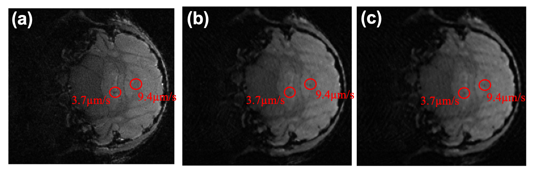
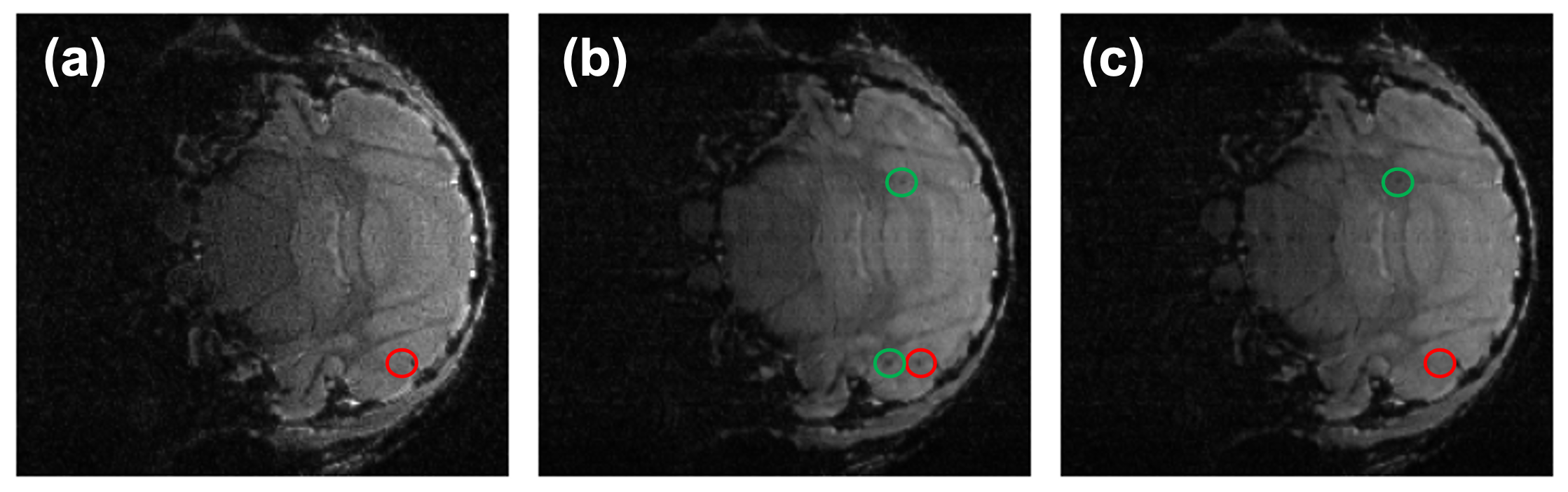
The method was first applied to simulated cell tracking experiments, where artificial cells of speeds 3.7 µm/s and 9.4 µm/s were added to an image of a mouse brain. The fully sampled image had best overall quality, as shown in Fig. 2a. However, the high-velocity cell could not be identified due to significant temporal blurring. With higher acceleration factors, the image quality decreased, but the cell features were more discernible. It is possible to combine the cell features detected in the high temporal resolution images with the low temporal resolution high quality background mouse brain in the image processing stage.
The method was then applied to in vivo data. Similar results were achieved, as shown in Fig. 3. The cell was not visible in the red highlighted region in the fully sampled image Fig. 3a (corresponding to the sampling pattern in Fig. 1a). The undersampled image had slightly reduced quality, but additional cells could be identified. Fig 3b was reconstructed with 21% of k-space data (corresponding to the 2nd frame in Fig. 1c) within the acquisition window of Fig. 3a, where a cell was visible in red. Fig. 3c was the time frame following Fig. 3b (corresponding to the 3rd frame in Fig. 1c), reconstructed with the same undersampling factor, where the cell in red had exited the slice. This indicated the cell was absent during approximately 60% of the acquisition time of Fig. 3a, leading to a negative detection in the fully sampled image. A few other cells that are visible in Fig. 3b&c, but not in Fig. 3a, are highlighted in green. This demonstrated how the sampling scheme improved the detection at virtually no cost.

Conclusion

We have presented a Cartesian sampling scheme for studying dynamic systems. Both the high temporal resolution images and fully sampled image are acquired. The undersampling ratio can be flexibly chosen retrospectively, providing a unique advantage when experimental conditions cannot be predetermined. Increased detection limits of cell velocity have been achieved with simulation and in vivo experiments.

Acknowledgements

M. A thanks Ontario Scholarship Program (Canada) for an OGS Scholarship. D. X. thanks NSERC Canada for a Discovery Grant.