1807
Three Dimensional Sodium Magnetic Resonance Fingerprinting using Irreducible Spherical Tensor Operator Simulations1Medical Physics in Radiology, German Cancer Research Center (DKFZ), Heidelberg, Germany, 2Center for Advanded Imaging Innovation and Research, New York University, New York, NY, United States, 3Center for Biomedical Imaging, Dept. of Radiology, New York University, New York, NY, United States, 4Physikalisch Technische Bundesanstalt (PTB), Braunschweig and Berlin, Germany, 5Institute of Radiology, University Hospital Erlangen, Friedrich-Alexander-Universität Erlangen (FAU), Erlangen, Germany
Synopsis
Sodium relaxation times have been shown to be altered in several diseases. Hence, 2D sodium relaxometry using Magnetic Resonance Fingerprinting (23Na-MRF) was demonstrated recently as a proof of concept. In this work an extension to a 3D sequence is presented. Furthermore, a more complex signal model based on irreducible spherical tensor operators was investigated. The feasibility of simultaneous 3D quantification of T1, T2s*, T2l*, T2* and ΔB0 was demonstrated in phantom measurements.
Introduction
Recently the feasibility of sodium Magnetic Resonance Fingerprinting (23Na-MRF) was presented as a proof of concept1,2, enabling the simultaneous quantification of T1,T2s*,T2l*,T2* and ΔB0. Here, non-steady state conditions were generated via temporally varying flip angles (FAs) and sequence timings to generate a unique signal evolution for a given parameter set. In this work, 23Na-MRF was extended in two ways: Firstly, the coverage was changed from 2D to 3D, allowing for simultaneous quantification of T1,T2s*,T2l*,T2* and ΔB0 in a 3D volume within approximately the same measurement time. Secondly, irreducible spherical tensor operators (ISTOs) were exploited for the simulations, which allow a more sophisticated signal simulation for spin 3/2-nuclei.Methods
The 3D-radial implementation of the previously proposed 23Na-MRF sequence1 uses a variable non-selective excitation pulse followed by a variable echo time (Fig.1) and a density adapted center-out radial readout3. Subsequently, a gradient rewinder is played out and a 2π spoiler gradient is switched along the z-direction, followed by the next excitation pulse. Each time frame was acquired with 150 center-out spokes which are distributed equidistantly in k-space, whereas subsequent time frames were rotated via the 13th tiny golden angle4 to achieve full sampling over the entire measurement. The dictionary simulation was based on ISTOs as proposed by Hancu et al.5, which are based on spectral density parameters ($$$J_0\geq J_1\geq J_2$$$), the off-resonance ΔB0 and the residual quadrupolar moment ωq. Relaxation towards M0 was enabled6. Under the assumption that ωq is negligible, the relaxation times can be calculated as7:$$T_{1l}=\frac{1}{2J_2};T_{1s}=\frac{1}{2J_1} [1] $$
$$T_{2l}=\frac{1}{J_1+J_2};T_{2s}=\frac{1}{J_0+J_1} [2]$$
To introduce the apparent transverse relaxation T2* (T2l*,T2s* respectively) each parameter set (J0,J1,J2,ωq), with central off-resonance ΔB0, was simulated for an off-resonance range of $$$\overline{ΔB_0}=[ΔB_0-100,ΔB_0-99,...,ΔB_0+100]$$$ Hz. The resulting signal evolutions were interpolated onto a 0.5Hz grid and summed along the $$$\overline{ΔB_0}$$$-direction, weighted with a Lorentzian distribution pL. Different T2* values were constructed by varying the width of pL such that $$$T_2>T_2^*>0.4T_2$$$ ($$$T_{2l}>T_{2l}^*>0.6T_{2l}$$$ respectively) in 1ms steps.
The expected signal evolution of a 23Na inversion recovery (IR) experiment is given by:
$$S(t)=S_0(1-2(0.8e^{-t/T_{1l}}+0.2e^{-t/T_{1s}})) [3]$$
However, in literature T1 is mostly modelled monoexponentially since the separation of T1l and T1s based on fitting the inversion recovery signal curve is challenging. Therefore, the first order Taylor expansion of a biexponential function with $$$a+b=1$$$ is considered:
$$ae^{\overline{a}t}+be^{\overline{b}t}=a\sum_{n=0}^\infty \frac{(\overline{a}t)^n}{n!}+b\sum_{n=0}^\infty \frac{(\overline{b}t)^n}{n!}\approx(a+b)+a\overline{a}t+b\overline{b}t=1+(a\overline{a}+b\overline{b})t\approx \sum_{n=0}^\infty \frac{((a \overline{a}+b \overline{b})t)^n}{n!}=e^{(a \overline{a}+b \overline{b})t} [4]$$
Comparison with equation [3] yields:$$$a=0.8$$$,$$$\overline{a}=\frac{-1}{T_{1l}}$$$,$$$b=0.2$$$ and $$$\overline{b}=\frac{-1}{T_{1s}}$$$, resulting in the monoexponential estimate:
$$\frac{1}{T_1}=\frac{0.8}{T_{1l}}+\frac{0.2}{T_{1s}} [5]$$
The dictionary was simulated as follows:
1. Set parameter space: biexponential: T1=[20,21,…70]ms, T2l=[15,16,…60], T2s=[1.0,1.3,…14.8], ΔB0=[-50,-48,…50]Hz;
monoexponential: T1=[30,31,…90]ms, T2=T2l=T2s=[5,6,…80]ms, ΔB0=[-50,-48,…50]Hz
2. Calculate T1l and T1s using equations [1],[2] and [5]
3. Delete parameter sets that violate $$$T_{1l} \geq T_{2l} \geq T_{1s} \geq T_{2s}$$$ ($$$\widehat{=}J_0 \geq J_1 \geq J_2$$$)
4. Convert parameter sets into spectral density parameters using equations [1] and [2]
5. Simulate signal evolution for each parameter set
6. Interpolate along $$$\overline{ΔB_0}$$$-axis to a step size of 0.5Hz
7. Sum up signal evolutions weighted with variable pL along the $$$\overline{ΔB_0}$$$-axis such that $$$T_{2l}>T_{2l}^*>0.6 T_{2l}$$$ (monoexponential: $$$T_{2}>T_{2}^*>0.4 T_{2}$$$) ; T2l* (T2*) in 1ms steps; central ΔB0 = [-50,-48,…,50]Hz
8. Concatenate biexponential and monoexponential parts
9. Compress dictionary using singular value decomposition (SVD) up to rank 12
The reconstruction was performed via a low rank alternating direction method of multipliers approach8,1.
Measurements (resolution: 3x3x3mm3) were performed on a 7T whole-body system (Siemens,Germany) using a 23Na-birdcage coil (Rapid,Germany). A cylindrical phantom filled with 0.9% NaCl solution (compartment 0), containing seven vials with additional 1%-7% agar (compartments 1-7), was imaged. A reference T1 map was determined based on an IR sequence (sequence parameters in Fig.2). Transverse relaxation parameters were determined by fitting a multi-echo GRE dataset (Fig.3). The phase difference yielded reference ΔB0 maps (Fig.2) and B1+ was measured using the phase sensitive method9 (FA=90°;TR=185ms;TE=0.55ms). The combined reference scan time (excluding B1+) was 7h42min, whereas the 23Na-MRF data was acquired within 1h4min.
Mean and SD of all quantified relaxation times were calculated in all vials for each slice.
Results
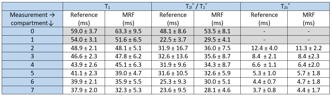
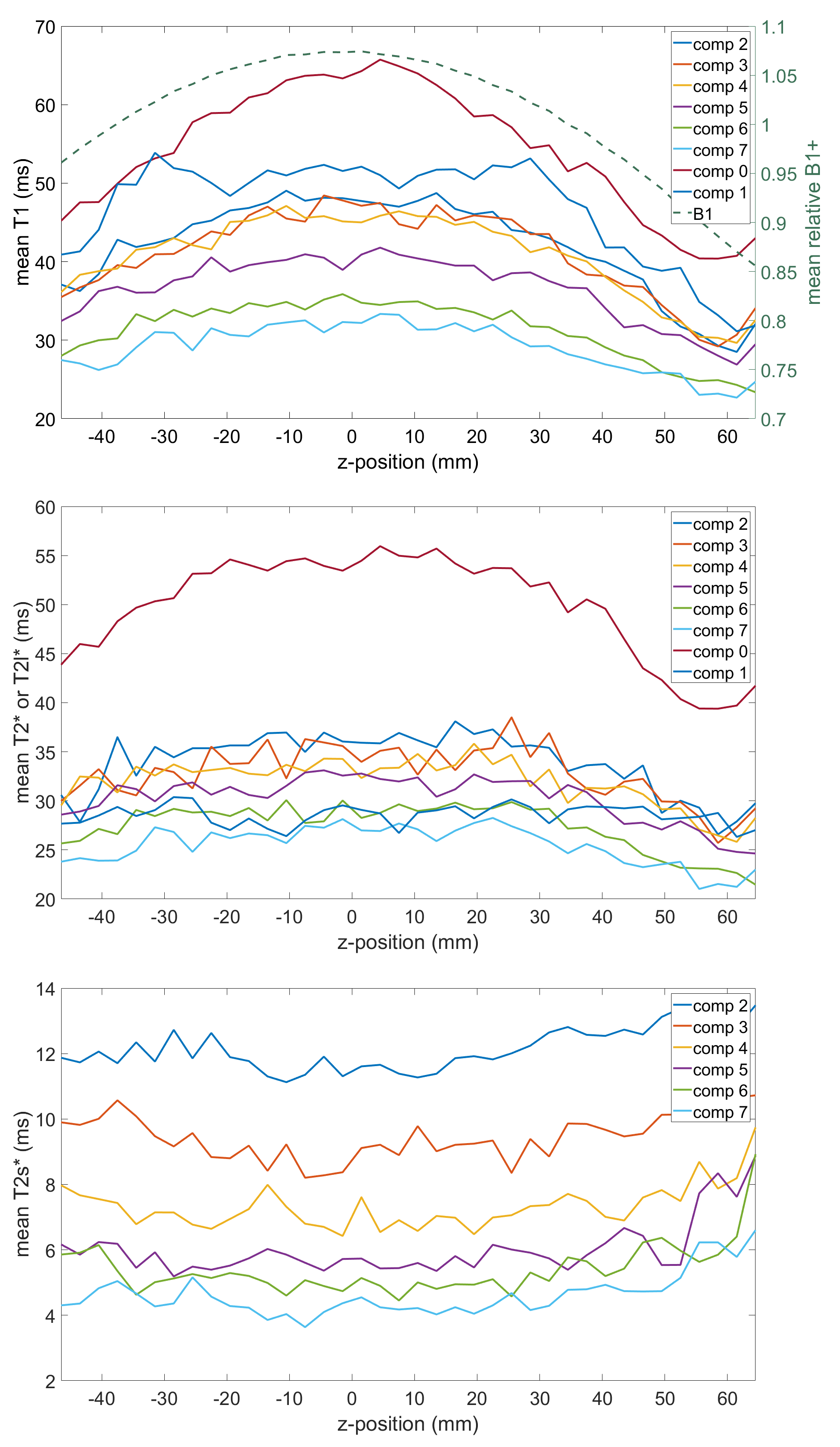
The resulting relaxation times and ΔB0 of the central slice are shown in Figs.2 and 3. All mean relaxation times obtained by 23Na-MRF are in agreement with the reference results within the SD (Tab.1), except for T1 in compartment 7 and T2* in compartment 1. Fig.4 displays the mean relaxation time in each compartment in dependence on the z-position, as well as the mean B1+ averaged over the whole phantom in each slice.Discussion and Conclusion
This work demonstrates the feasibility of simultaneously quantifying T1,T2s*,T2l*,T2* and ΔB0 within approximately 1h by means of 3D 23Na-MRF in combination with ISTOs for the dictionary simulation. Despite using a fairly simple FA and TE pattern, good agreement between the results of the reference measurements and 3D 23Na-MRF was found. The differences in T1 in compartment 7 can be explained as here strong a biexponential T1 could be present10, violating equations [4] and [5]. In compartment 1, T2* can be described both bi- and monoexponentially almost equally well (see Fig.3), which could explain the discrepancy between reference and MRF.Fig.4 indicates that B1+ correction could improve the parameter quantification.
These experiments are promising as this technique could allow full 3D-mapping of the relaxometric parameters in less than 1h.
Acknowledgements
No acknowledgement found.References
1. Kratzer FJ, Flassbeck S, Nagel AM, Behl NGR, Knowles BR, Bachert P, Ladd ME, Schmitter S. Sodium relaxometry using 23Na MR fingerprinting: A proof of concept. Magn Reson Med. 2020; 84(5):2577-2591
2. Kratzer FJ, Schmitter S, Nagel AM, Behl NGR, Knowles BR, Bachert P, Ladd ME, Flassbeck S. Sodium Relaxometry using Magnetic Resonance Fingerprinting. Proc. ISMRM 2020. #0392
3. Nagel AM, Laun FB, Weber MA, Matthies C, Semmler W, Schad LR. Sodium MRI Using a Density-Adapted 3D Radial Acquisition Technique. Magn Reson Med 2009; 62: 1565-1573
4. Frydahl A, Holst K, Caidahl K, Ugander M, Sigfridsson A. Generalization of three-dimensional golden-angle radial acquisition to reduce eddy current artifacts in bSSFP CMR imaging. MAGMA. 2020. doi: 10.1007/s10334-020-00859-z
5. Hancu I, Van der Maarel J, Boada F. A Model for the Dynamics of Spins 3/2 in Biological Media: Signal Loss during Radiofrequency Excitation in Triple-Quantum-Filtered Sodium MRI. Journal of Magnetic Resonance 2000; 147(2):179-191
6. Stobbe R, Beaulieu C. In Vivo Sodium Magnetic Resonance Imaging of the Human Brain Using Soft Inversion Recovery Fluid Attenuation. Magn Reson Med 2005; 54:1305-1310
7. Van der Maarel J. Thermal relaxation and coherence dynamics of spin 3/2. I. Static and fluctuating quadrupolar interactions in the multipole basis. Concepts in MR 2003; 19A(2): 97-116
8. Asslander J, Cloos MA, Knoll F, Sodickson DK, Hennig J, Lattanzi R. Low rank alternating direction method of multipliers reconstruction for MR fingerprinting. Magn Reson Med 2018;79(1):83-96
9. Morrel GR. A phase-sensitive method of flip angle mapping. Magn Reson Med 2008;60(4):889-894
10. Wilferth T, Gast LV, Stobbe RW, Beaulieu C, Hensel B, Uder M, Nagel AM. 23Na MRI of human skeletal muscle using long inversion recovery pulses. Magn Resin Imag 2019;63:280-209
Figures
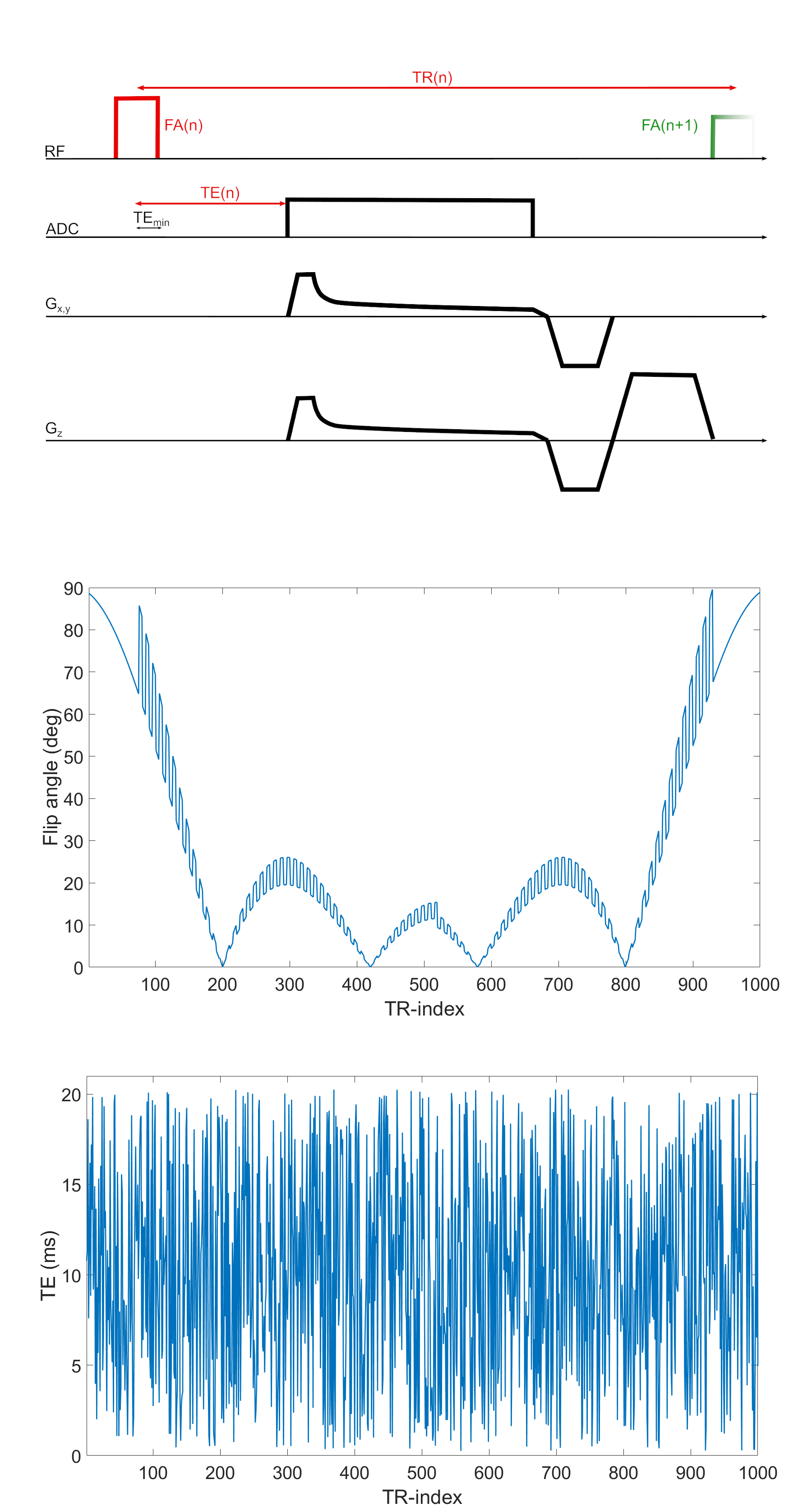
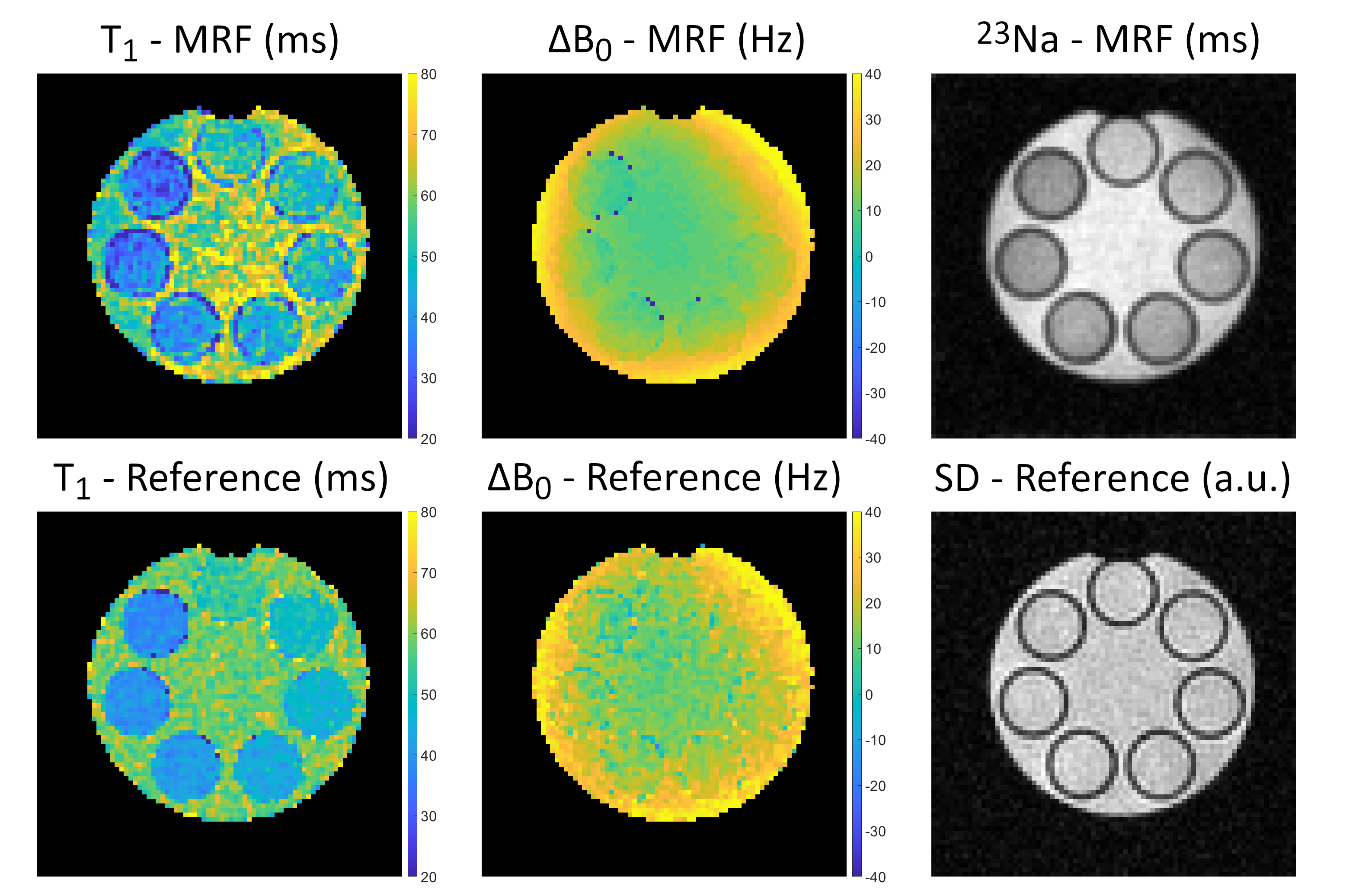
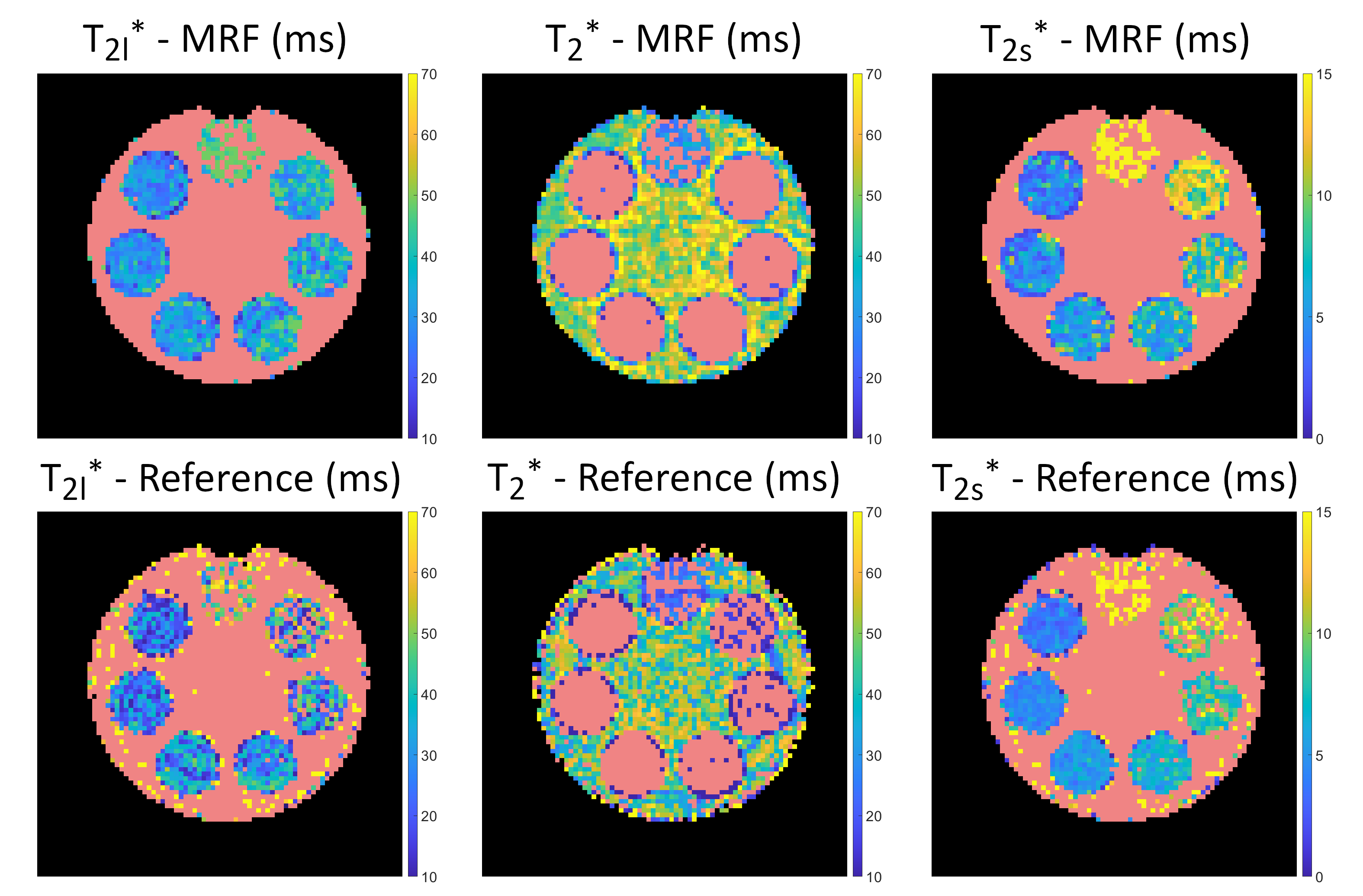
Fig.3: Phantom measurements of the transverse relaxation acquired with MRF (top) and the reference method (bottom). Here, both a mono- and a biexponential FID were fitted to multi-echo GRE images (FA=90°;TR=200ms;TE: 32 samples in [0.35,54.6]ms;Tacq=1h47min). The red masks in the T2l* and T2s* maps indicate pixels that were determined to relax monoexponentially (biexponentially in T2* maps). For the reference measurement, this distinction was determined by the goodness of the fit R2, whereas MRF determined this differentiation intrinsically in the dictionary matching step.