1778
Fine-tuning deep learning model parameters for improved super-resolution of dynamic MRI with prior-knowledge1Biomedical Magnetic Resonance, Otto von Guericke University, Magdeburg, Germany, 2Institute for Medical Engineering, Otto von Guericke University, Magdeburg, Germany, 3Data and Knowledge Engineering Group, Otto von Guericke University, Magdeburg, Germany, 4Faculty of Computer Science, Otto von Guericke University, Magdeburg, Germany, 5Center for Behavioral Brain Sciences, Magdeburg, Germany, 6German Center for Neurodegenerative Disease, Magdeburg, Germany, 7Leibniz Institute for Neurobiology, Magdeburg, Germany
Synopsis
Dynamic imaging is required during interventions to assess the physiological changes. Unfortunately, while achieving a high temporal resolution the spatial resolution is compromised. To overcome the spatiotemporal trade-off, in this work deep learning based super-resolution approach has been utilized and fine-tuned using prior-knowledge. 3D dynamic data for three subjects was acquired with different parameters to test the generalization capabilities of the network. Experiments were performed for different in-plane undersampling levels. A U-net based model[1] with perceptual loss[2] was used for training. Then, the trained network was fine-tuned using prior scan to obtain high resolution dynamic images during the inference stage.
Introduction
The use of dynamic MRI is crucial for abdominal interventions such as liver [3-4]. However, conventional rapid imaging suffers from a trade-off between spatial and temporal resolution, preventing usage in clinical routines. Super-resolution (SR) is a class of algorithms that intends to provide a high resolution image from a low resolution counterpart and has been broadly used in many tasks [5-6]. In an earlier work [7], SR was shown to be a promising tool to improve the spatiotemporal trade-off in dynamic MRI. Owing to the requirement of respiratory navigation and post-processing to stack all slices in 2D dynamic scan, that investigation was extended using 3D dynamic datasets to obtain high spatiotemporal resolution output. The dynamic images were considered as separate 3D volumetric images at different time points, referred to as 3D+t imaging.Methods
A. Data Preparation3D abdominal dynamic acquisitions of three healthy subjects were acquired on a 3T scanner (SIEMENS MAGNETOM Skyra) and were artificially undersampled in-plane using MRUnder [8] pipeline to simulate low resolution data. To test the generalization of the network, the dynamic acquisitions were obtained using T1w FLASH but with varied sequence parameters, as illustrated in Table 1. The undersampling was done by taking the central part along the phase encoding direction of the k-space and then cropped with the aspect ratio of the image without zero-padding. The different levels of undersampling (us 25% and us 10% of the k-space) were investigated. In this work, CHAOS challenge [9] data was used for the main training. Fig. 1 shows the schematic diagram of the proposed method along with the network architecture.
B. Model Implementation and Training
For the main training, 243 patches with a stride of six for the slice dimension and 12 for the other dimensions were chosen from the CHAOS dataset. Next, the trained-model was fine-tuned using the first time point (t0) of different 3D+t acquisitions, considering them as the planning scans. The patch size of 243 and stride of one were selected for the fine-tuning step. The perceptual loss [9] was used to calculate the loss during training and fine-tuning. The output loss at each level of a pre-trained perceptual loss network [10] was calculated using L1 loss. The implementation was done with PyTorch and was trained using Nvidia Tesla V100 GPUs. Adam optimizer with a learning rate of 1e-4 was used for the main training, and was trained for 200 epochs. The network was fine-tuned for one epoch utilizing the planning scan with a lower learning rate of 1e-6.
Results
Fig. 2 portrays the highest percentage of undersampling with the same slices from different time points. The low resolution inputs, trilinear interpolated images, super-resolution results of the main training, super-resolution results after fine-tuning, and the ground-truth images are shown in this figure for visual comparison. Fig. 3 displays the reconstructed results (before and after fine-tuning) compared against the ground-truth for undersampled 10%. The two ROIs highlighted in yellow and red are illustrated using zoomed-in images. Each reconstructed results as well as their difference to the ground-truth are shown. For quantitative evaluation between two different undersampling levels, Table 2 illustrates the average of SSIM, PSNR, and the standard deviation (SD) of the difference images of all time points for all dynamic datasets.Discussions
In brief, fine-tuning the SR with priors is promising in mitigating the spatiotemporal tradeoff in dynamic MRI. While using the highly undersampled data, there was a noticeable improvement visually and numerically. The fine-tuned model could also mitigate the undersampling artefacts, which the main training without a priori-data could not. The input k-space was zero-padded for comparison, resulted in a higher SSIM than trilinear. In addition, one can observe that the network performed better in restoring the small details particularly at the anterior and posterior of the abdomen. It is to be noted that in this study, the network was trained using MR images of different sequences other than the dynamic data (CHAOS: T1 in- and opposed phases and T2 SPIR, 3D dynamic acquisition: T1w FLASH) but still yielded promising results. Therefore, employing SR incorporated with priors allows the journey beyond the spatiotemporal trade-off in dynamic MRI. The fast inference speed of the SR predictions allows the application in real-time diagnostics. In further investigation, the feasibility of higher accelerated acquisitions of the dynamic data and the optimization of the hyperparameters such as the learning rate of the fine-tuning step will be evaluated. Moreover, the assessment in a larger number of subjects to use in clinical diagnostic will also be tested.Acknowledgements
This work was conducted within the context of the International Graduate School MEMoRIAL at Otto von Guericke University (OVGU) Magdeburg, Germany, kindly supported by the European Structural and Investment Funds (ESF) under the programme "Sachsen-Anhalt WISSENSCHAFT Internationalisierung“ (project no. ZS/2016/08/80646).References
1. Ronneberger, Olaf, Philipp Fischer, and Thomas Brox. "U-net: Convolutional networks for biomedical image segmentation." International Conference on Medical image computing and computer-assisted intervention. Springer, Cham, 2015.
2. Johnson, Justin, Alexandre Alahi, and Li Fei-Fei. "Perceptual losses for real-time style transfer and super-resolution." European conference on computer vision. Springer, Cham, 2016.
3. Rempp, Hansjörg, et al. "MR-guided radiofrequency ablation using a wide-bore 1.5-T MR system: clinical results of 213 treated liver lesions." European radiology 22.9 (2012): 1972-1982.
4. Moche, Michael, et al. "Navigated MRI-guided liver biopsies in a closed-bore scanner: experience in 52 patients." European radiology 26.8 (2016): 2462-2470.
5. Dong, Chao, et al. "Learning a deep convolutional network for image super-resolution." European conference on computer vision. Springer, Cham, 2014.
6. Huang, Yawen, Ling Shao, and Alejandro F. Frangi. "Simultaneous super-resolution and cross-modality synthesis of 3D medical images using weakly-supervised joint convolutional sparse coding." Proceedings of the IEEE Conference on Computer Vision and Pattern Recognition. 2017.
7. Sarasaen, Chompunuch, Chatterjee, Soumick, Nürnberger, Andreas and Speck, Oliver, “Super Resolution of Dynamic MRI using Deep Learning, Enhanced by Prior-Knowledge.” Magnetic Resonance Materials in Physics, Biology and Medicine, 33(Supplement 1): S03.04, S28-S29, 2020.
8. Soumick Chatterjee. (2020, June 19). soumickmj/MRUnder: Initial Release (Version v0.1). DOI: http://doi.org/10.5281/zenodo.3901455
9. Kavur, A. Emre, et al. "CHAOS Challenge--Combined (CT-MR) Healthy Abdominal Organ Segmentation." arXiv preprint arXiv:2001.06535 (2020).
10. Chatterjee, Soumick, et al. "DS6: Deformation-aware learning for small vessel segmentation with small, imperfectly labeled dataset." arXiv preprint arXiv:2006.10802 (2020).
Figures
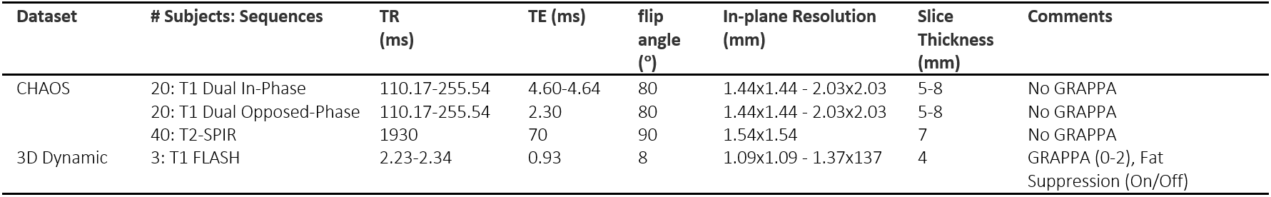
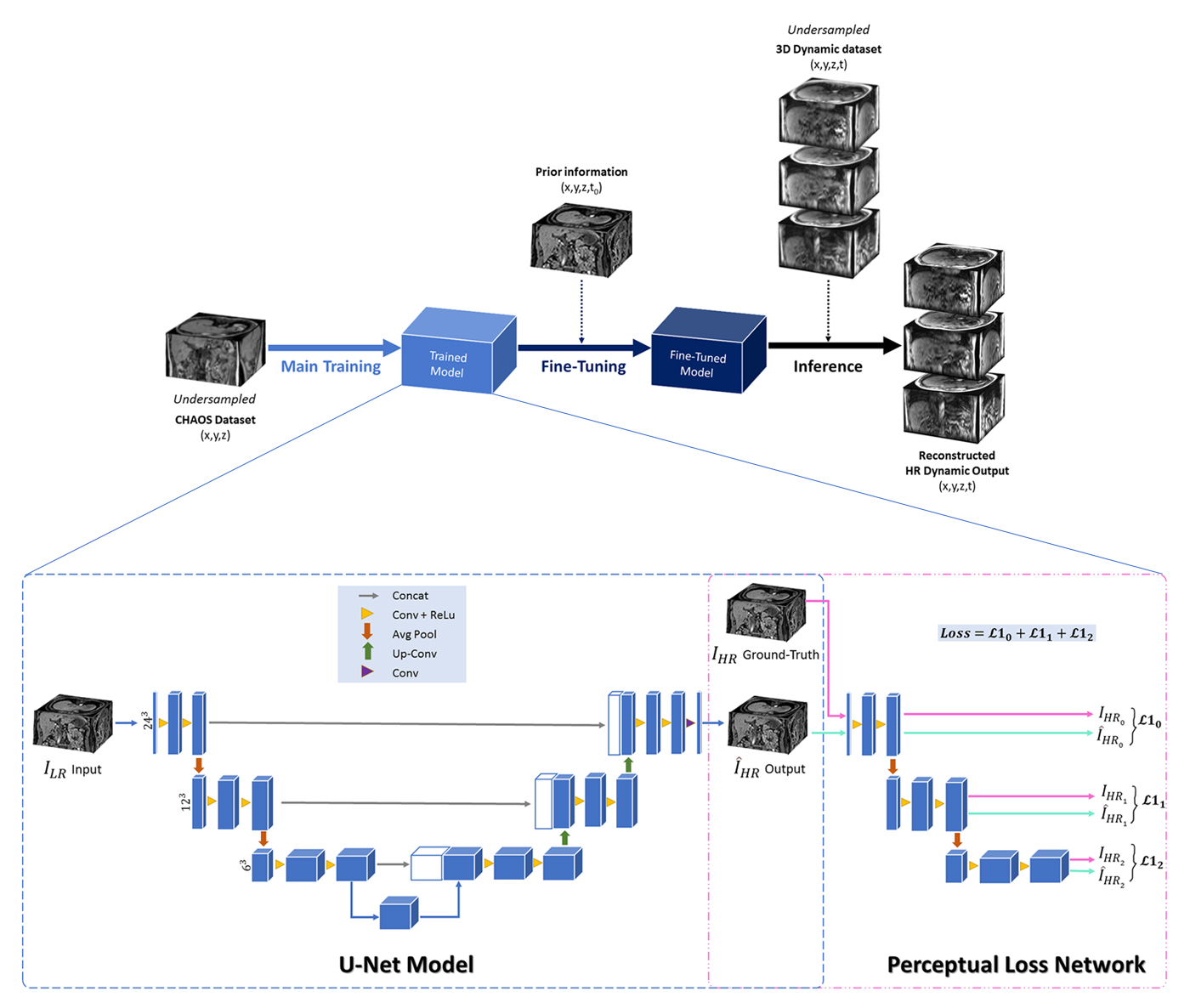
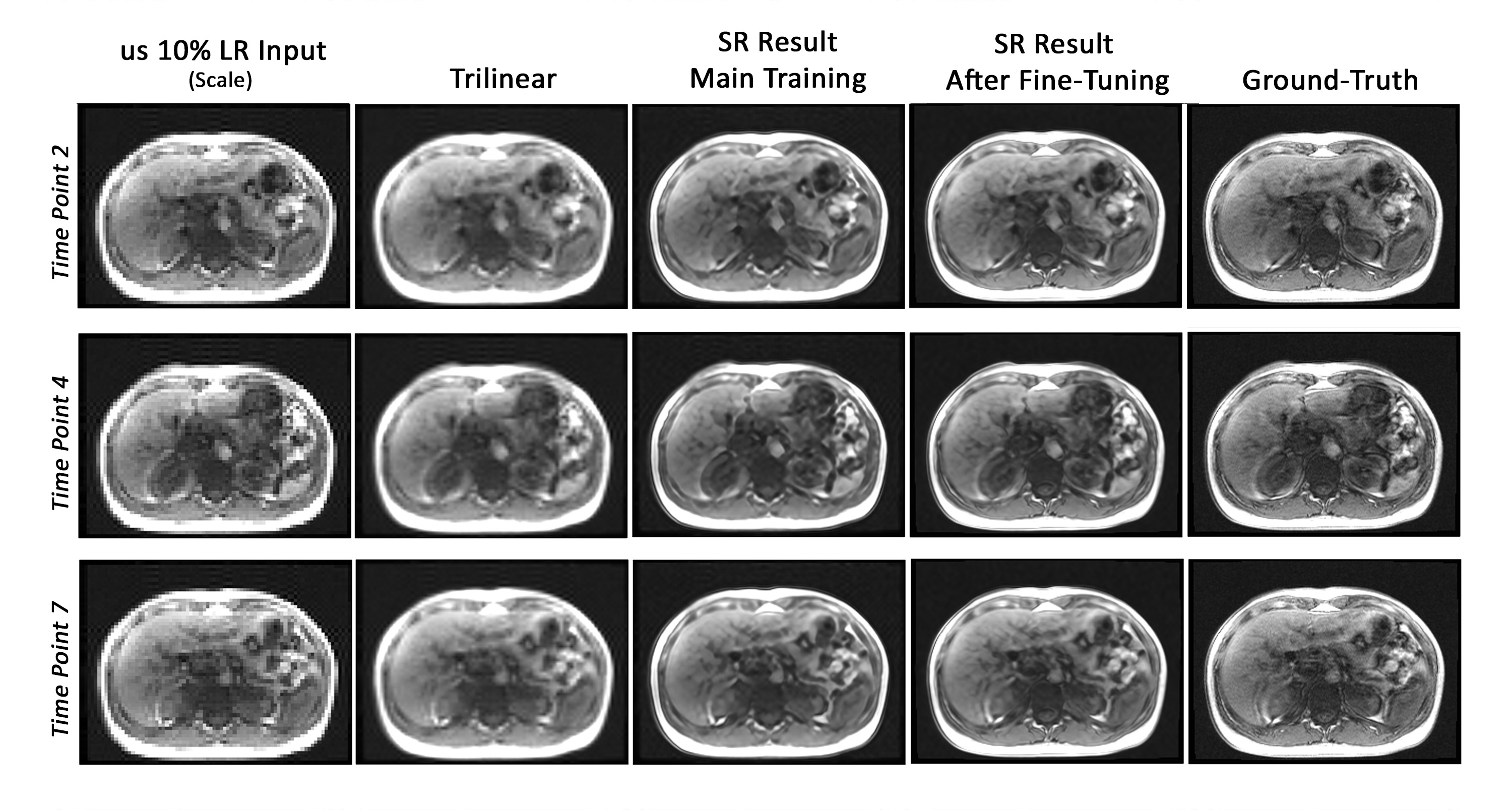
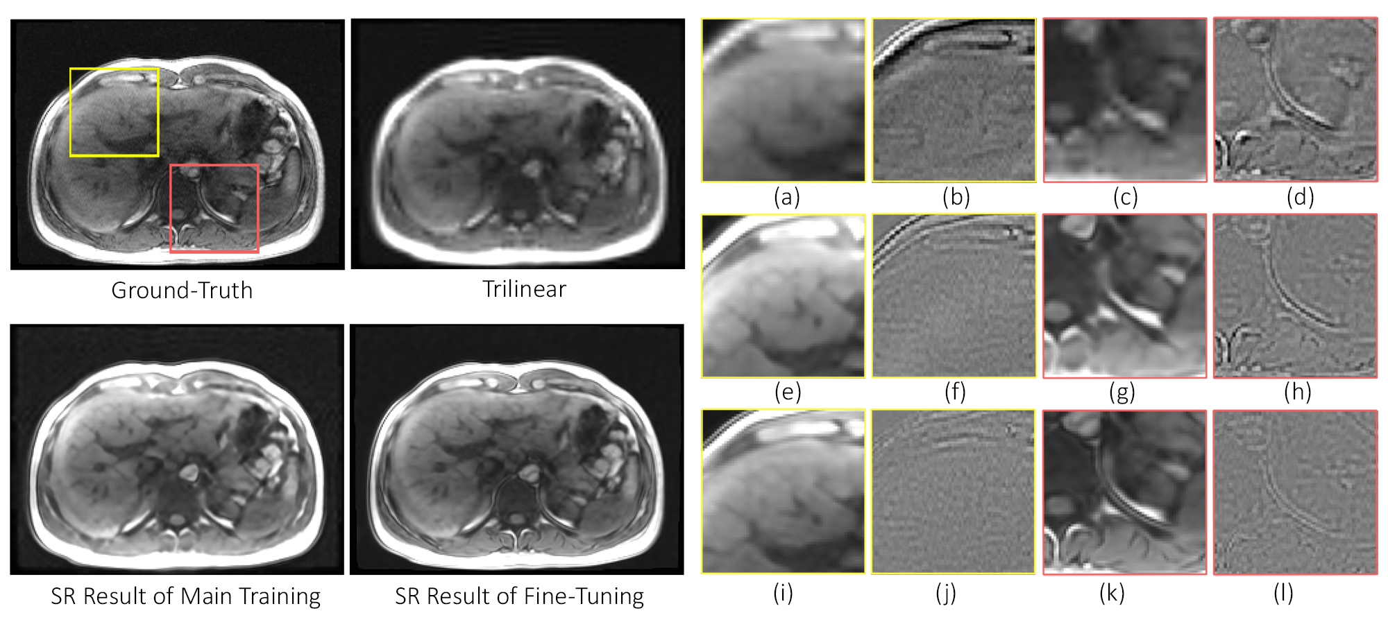
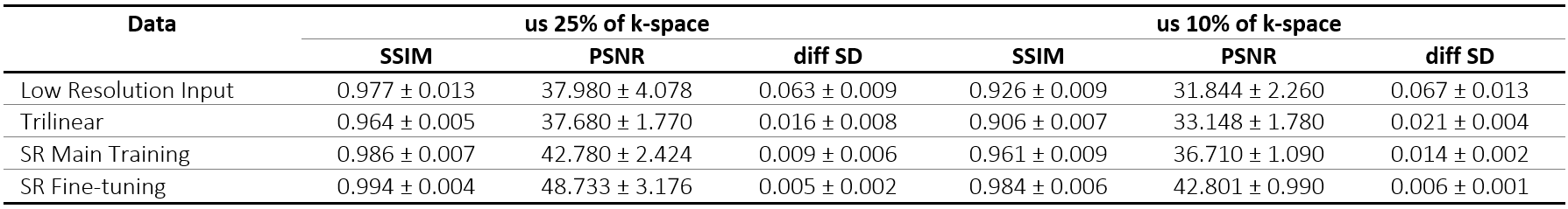
Table 2 The average of SSIM, PSNR, and the standard deviation (SD) of the difference images of all time points for all dynamic datasets. The table shows the result of undersampled 25% and 10% of the k-space.