Introduction

Image reconstruction using a priori constraints, such as sparsity, low-rankness, and machine learning priors has become popular in recent years.^1-3 The underlying regularization problem requires selection of good regularization parameters to produce high-quality images. Conventional methods often either use empirical values or apply statistical testing such as L-curve,^4-5 cross-validation^6-7 and SURE,^8-9 to determine those parameters, which is computationally expensive. In this work, we propose a novel deep learning-based approach to solve this fundamental problem associated with constrained reconstruction. We use neural networks (NN) to learn such manifolds from training data and apply them to determine the optimal regularization parameters for newly acquired images in a computationally efficient way. Experimental studies have been performed to evaluate the proposed method.

Methods

Most constrained reconstruction problems in MRI can be formulated as:
$$\hspace{10em}\widehat{\rho}=\arg \min_{\rho} ||d-E\rho||_2^2+\sum_{i=1}^n\lambda_iR_i(\rho)\hspace{10em}(1)$$
where $$$\rho$$$ denotes the desired image function, $$$d$$$ measured data, $$$\small{E}$$$ imaging operator, $$$\small{R_{i}(\cdot)}$$$ regularization functions, and $$$\small{\lambda_{i}}$$$ regularization parameters. The paper addresses the problem of optimal selection of $$$\small{\left\{\lambda_{i}\right\}}$$$ using a learning (instead of statistical testing) based method.

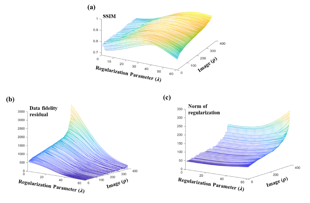
The proposed method exploits the fact that given $$$\small{E}$$$, $$$\small{R_{i}(\cdot)}$$$ and a class of images, most of the image quality metrics (e.g., L-curve), as a function of $$$\small{\left\{\lambda_{i}\right\}}$$$ and $$$\rho$$$, form low-dimensional manifolds $$$\small{M(\left\{\lambda_{i}\right\}, \rho)}$$$. These low-dimensional manifolds, as illustrated in Fig. 1, can be learnt and then used for prediction for a new data set. With these predicted metrics, the optimal values for $$$\small{\left\{\lambda_{i}\right\}}$$$ are then determined by NN trained using ground truth data. In our current implementation, two image quality manifolds were learnt from training data: a) SSIM (structural similarity index measure), $$$\small{M_{\text{SSIM}}(\left\{\lambda_{i}\right\}, \rho)}$$$, and b) L-curve, $$$\small{M_{\text{Lcurve}}(\left\{\lambda_{i}\right\}, \rho)}$$$, that measures the tradeoff between data fidelity and regularization.

For a given $$$\rho$$$, if we know the solutions, $$$\small{\widehat{\rho}_{m}}$$$, to Eq.(1) for a set of values of the regularization parameters, say, $$$\small{\left\{\lambda_{i}(m)\right\}_1^M}$$$, within their permissible range, $$$\small{M_{\text{Lcurve}}(\left\{\lambda_{i}(m)\right\}, \widehat{\rho}_{m})}$$$ can be calculated easily; $$$\small{M_{\text{SSIM}}(\left\{\lambda_{i}(m)\right\}, \widehat{\rho}_{m})}$$$ can also be determined if a reference $$$\small{{\rho}_{\text{ref}}}$$$ is available. However, solving Eq.(1) for $$$\small{\left\{\lambda_{i}(m)\right\}_1^M}$$$ to determine $$$\small{\widehat{\rho}_{m}}$$$ is computationally expensive and thus not feasible practically.

We solved this problem using a machine learning-based method. More specifically, we solved Eq. (1) for only a few values from $$$\small{\left\{\lambda_{i}(m)\right\}_1^M}$$$ , say $$$n+1$$$ values with $$$n$$$ being the number of regularization terms in Eq. (1). With these reconstructions, we used an interpolation method to generate $$$\small{\widehat{\rho}_{m}^0}$$$. Interestingly, while $$$\small{\widehat{\rho}_{m}^0}$$$ are rather poor approximations of $$$\small{\widehat{\rho}_{m}}$$$, we can train a neural network to map $$$\small{M_{\text{Lcurve}}(\left\{\lambda_{i}(m)\right\},\widehat{\rho}_{m}^0)}$$$ to $$$\small{M_{\text{Lcurve}}(\left\{\lambda_{i}(m)\right\}, \widehat{\rho}_{m})}$$$. Similarly, we can also train a network to map $$$\small{M_{\text{SSIM}}(\left\{\lambda_{i}(m)\right\}, \widehat{\rho}_{m}^0)}$$$ to $$$\small{M_{\text{SSIM}}(\left\{\lambda_{i}(m)\right\}, \widehat{\rho}_{m})}$$$ using references generated from $$$\small{\widehat{\rho}_{m}^0}$$$ by another network. Here, we used a generative adversarial network to produce the references, which was trained with ground truth data; we used two fully-connected networks to predict SSIM and L-curve, which were trained using training data with pre-calculated quality metrics for both $$$\small{\widehat{\rho}_{m}}$$$ and $$$\small{\widehat{\rho}_{m}^0}$$$. With SSIM and L-curve predicted, we fused them to produce the final estimate of $$$\small{\left\{\lambda_{i}\right\}}$$$ using a fully-connected network.

It is important to note that instead of directly learning the manifolds from the initial reconstructions $$$\small{\widehat{\rho}_{m}^0}$$$ or learning $$$\small{\widehat{\rho}_{m}}$$$ from $$$\small{\widehat{\rho}_{m}^0}$$$, we converted them to the initial quality metrics $$$\small{M_{\text{Lcurve}}(\left\{\lambda_{i}(m)\right\},\widehat{\rho}_{m}^0)}$$$ and $$$\small{M_{\text{SSIM}}(\left\{\lambda_{i}(m)\right\},\widehat{\rho}_{m}^0)}$$$ , thus significantly reducing the learning complexity and enhancing the quality of the predicted results of the trained networks. Also, as compared to the traditional L-curve method, the proposed method incorporates both $$$\small{M_{\text{Lcurve}}}$$$ and $$$\small{M_{\text{SSIM}}}$$$, thus enabling more optimal parameter selection.

Results

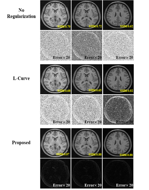
The proposed method was tested in three reconstruction scenarios: image deblurring, parallel imaging, and dynamic image denoising. The first two problems entailed one regularization term, absorbing spatial smoothness constraint; the third application involved two regularization terms imposing low-rankness and sparsity constraints, respectively.

For image deblurring, the measured data were simulated using T1W images from HCP database with a Gaussian smoothing kernel plus random noise. Figure 2 shows the reconstruction results using the regularization parameters selected by L-curve and the proposed method. As can be seen, our method led to much better reconstruction quality in much shorter processing time (L-Curve: 3s, Proposed: 0.1s per slice).

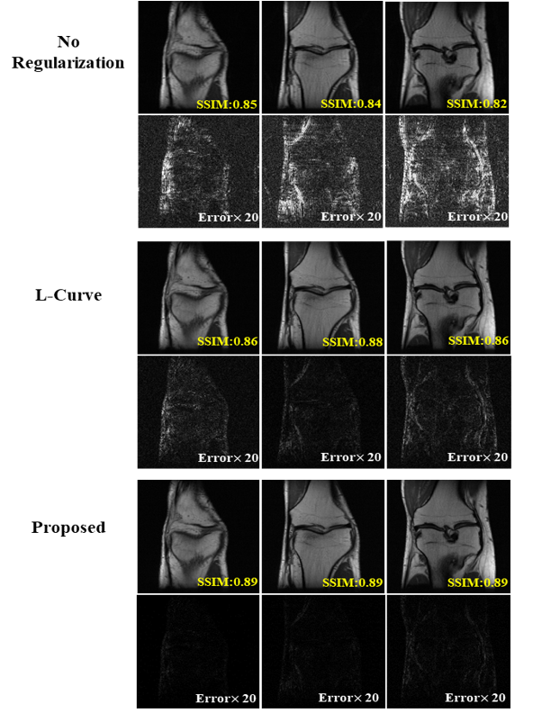
For parallel imaging, we used the multi-coil knee data from the NYU database with retrospective undersampling (R=2.5). The results are summarized in Fig. 3. As can be seen, our method achieved superior performance over the traditional L-curve method.

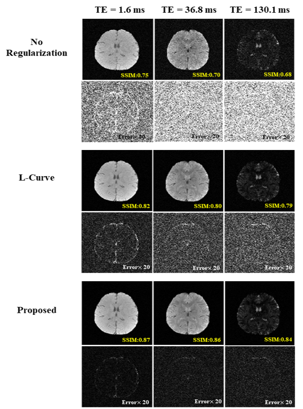
For dynamic image denoising, a series of $$$\small{\text{T}_2^*\text{W}}$$$ images were acquired using the mGRE sequence with 74 echoes. Gaussian noise was also added retrospectively to produce a range of SNR levels. The reconstruction results are shown in Fig. 4. Note our method handled the reconstruction problem well even with multiple regularization parameters that are very challenging to be determined optimally and efficiently using traditional statistical testing-based methods.

Conclusion

We have proposed a novel learning-based method for efficient selection of optimal regularization parameters for constrained image reconstruction. Our method has been evaluated using experimental data, producing very encouraging results. The proposed method may help improve the effectiveness and practical utility of constrained reconstruction.

Acknowledgements

This work was supported in a part by National Natural Science Foundation of China (62001293)