1764
ArtifactID: identifying artifacts in low field MRI using deep learning
Marina Manso Jimeno1,2, Keerthi Sravan Ravi2,3, John Thomas Vaughan Jr.2,3, Dotun Oyekunle4, Godwin Ogbole4, and Sairam Geethanath2
1Biomedical Engineering, Columbia University, New York, NY, United States, 2Columbia Magnetic Resonance Research Center (CMRRC), New York, NY, United States, 3Columbia University, New York, NY, United States, 4Radiology, University College Hospital, Ibadan, Nigeria
1Biomedical Engineering, Columbia University, New York, NY, United States, 2Columbia Magnetic Resonance Research Center (CMRRC), New York, NY, United States, 3Columbia University, New York, NY, United States, 4Radiology, University College Hospital, Ibadan, Nigeria
Synopsis
Most MR images contain artifacts such as wrap-around and Gibbs ringing, which negatively affect the diagnostic quality and, in some cases, may be confused with pathology. This work presents ArtifactID, a deep learning based tool to help MR technicians to identify and classify artifacts in datasets acquired with low-field systems. We trained binary classification models to accuracies greater than 88% to identify wrap-around and Gibbs ringing artifacts in T1 brain images. ArtifactID can help novice MR technicians in low resource settings to identify and mitigate these artifacts.
Introduction
Most MR images contain artifacts [1, 2] such as wrap-around, Gibbs ringing, etc. These artifacts negatively affect the diagnostic quality and, in some cases, may be confused with pathology [1]. Identifying artifacts requires expertise, and eliminating them demands prior knowledge of their source and underlying phenomena [3]. Developing countries witness scarcity of skilled MR technicians and radiologists [4, 5]. This scarcity results in avoidable scan repetitions, increased operating time and costs [6, 7], and occasionally misdiagnosis and misinterpretation. In this work, we demonstrate ArtifactID as a first step in the solution to this challenge of identifying artifacts in brain MRI. ArtifactID can identify wrap-around and Gibbs ringing artifacts occurring in data acquired from 0.36T field strengths.Methods
We synthesized wrap-around utilizing the publicly available IXI dataset [8] (T1 contrast only). Patches containing the edges of the volume across all three axes were extracted from each input slice and overlaid onto the central region. The simulation code chose the patch’s extent at random in the range [5, 35] and set the overlaid patch’s opacity to 75%. We combined real-world low-field (0.36T) pathological brain volumes with the simulated data for the validation and testing sets. For Gibbs ringing, the artifact simulation process employed only low-field data instead of a publicly available dataset. We manually chose brain slices not containing the artifact based on visual inspection. The simulation process involved removing a contiguous block of k-space lines along the input image’s phase-encode direction. We randomized the number of lines to delete and the block’s starting location at random in the range [32, 64] and [0, 160]. Figure 1 shows representative slices of simulated and low-field data for each simulated artifact. The dataset combined the simulated data and natively corrupted data. Data-preprocessing of both artifacts resized each slice to size 256 x 256 and normalized pixel intensities to lie in the range [0, 1]. We trained a binary classification model for each artifact identification task. The low-field, neuro-radiologist labeled images were obtained from a 0.36T scanner at University College Hospital, Ibadan, Nigeria. Figure 2 presents the dataset-splits utilized in this work. Figure 3 shows the 2D convolutional network architecture designed using TensorFlow-Keras [9] and provides training details. The entire source code is open-source and available on Github [10].Results
Training the wrap-around artifact identification model for 10 epochs required approximately 12 minutes to achieve training/validation accuracies of 94% and 88%. Precision and recall metrics evaluated on the validation and test sets were 91.7%/82.6% and 89.7%/86.7% respectively. Figure 4A shows the corresponding confusion matrices. We used the validation results to tweak the simulation parameters and optimize artifact fidelity. Filter visualization (Figure 4B) of a true-positive (TP), true-negative (TN), false-positive (FP), and false-negative (FN) indicates that the model is learning to identify the overlap of volumes that occurs on wrap-around artifacted images. For training the Gibbs artifact identification model, we replaced the publicly available IXI dataset with low-field data. The reason was inherent contrast differences observed in prior experiments comparing data acquired from low-field and high-field scanners. Training the model for 100 epochs required approximately 4.41 minutes. The models achieved training/validation accuracies of 89.5% and 94%. The precision and recall metrics computed on the validation and test sets were 100%/90.9% and 86.6%/79.2%. Figure 4B shows the relevant confusion matrices.Discussion and conclusion
Low-field MRI scanners are more accessible in resource-limited regions [5,11], where personnel may lack the required knowledge to accurately o identify and correct artifacts. Images acquired from low-field systems are inherently prone to certain artifacts [11]. We have demonstrated the application of deep-learning-based methods to identify wrap-around and Gibbs ringing artifacts in low-field images. We utilized a simple 2D CNN architecture to learn the artifacts from simulated and real-world images at 3T and 0.36T field strengths. The preliminary results indicate that the networks can identify the artifacts with 89.5% accuracy and above across both identification tasks. For model explainability purposes, we visualized filter activations for brain slices from the low-field dataset. Figures 4 and 5 show the most representative filters. For wrap-around artifact identification (Figure 4), the background volumes in both the TP and FP similarly excite the filters. In the case of the TP, the background volume corresponds to the overlaid slice. The TN example doesn’t show any background activation. In the FN case, the overlaid wrap activates differently from the TP, which might have led to incorrect classification. For Gibbs ringing artifact identification (Figure 5), visualizing filter activations was inconclusive since the model acted on frequency-domain input. As future work, we will test ArtifactID in a deployment scenario for prospective use. We will also increase the artifact dossier to include low SNR images, motion artifacts, etc. We will provide recommendations to mitigate the identified artifact if image re-acquisition is an option. In conclusion, this tool will help the MR technician identify possible artifacts in the data that may interfere with diagnosis on-site at the scan time. We believe this is a valuable feature that would help mitigate artifacts.Acknowledgements
This study was funded [in part] by the Seed Grant Program for MR Studies and the Technical Development Grant Program for MR Studies of the Zuckerman Mind Brain Behavior Institute at Columbia University and Columbia MR Research Center site.References
- K. Krupa and M. Bekiesińska-Figatowska, “Artifacts in magnetic resonance imaging,” Polish J. Radiol., 2015.
- T. B. Smith and K. S. Nayak, “MRI artifacts and correction strategies,” Imaging Med., vol. 2, no. 4, pp. 445–447, 2010.
- M. J. Graves and D. G. Mitchell, “Body MRI artifacts in clinical practice: A physicist’s and radiologist’s perspective,” J. Magn. Reson. Imaging, vol. 38, no. 2, pp. 269–287, 2013.
- G. I. Ogbole, A. O. Adeyomoye, A. Badu-Peprah, Y. Mensah, and D. A. Nzeh, “Survey of magnetic resonance imaging availability in West Africa,” Pan Afr. Med. J., 2018.
- S. Geethanath and J. T. Vaughan, “Accessible magnetic resonance imaging: A review,” J. Magn. Reson. Imaging, vol. 49, no. 7, pp. 65–77, 2019.
- J. B. Andre et al., “Toward Quantifying the Prevalence, Severity, and Cost Associated With Patient Motion During Clinical MR Examinations,” J. Am. Coll. Radiol., vol. 12, no. 7, pp. 689–695, Jul. 2015.
- M. A. Hossain, M. Ahmad, M. R. Islam, and M. A. Rashid, “Improvement of Medical Imaging Equipment Management in public hospitals of Bangladesh,” in 2012 International Conference on Biomedical Engineering, ICoBE 2012, 2012.
- https://brain-development.org/ixi-dataset/
- M. Abadi et al., “TensorFlow: A system for large-scale machine learning,” in Proceedings of the 12th USENIX Symposium on Operating Systems Design and Implementation, OSDI 2016, 2016.
- https://github.com/imr-framework/artifactID
- G. Ogbole, J. Odo, R. Efidi, R. Olatunji, and A. Ogunseyinde, “Brain and spine imaging artefacts on low-field magnetic resonance imaging: Spectrum of findings in a Nigerian Tertiary Hospital,” Niger. Postgrad. Med. J., 2017.
Figures
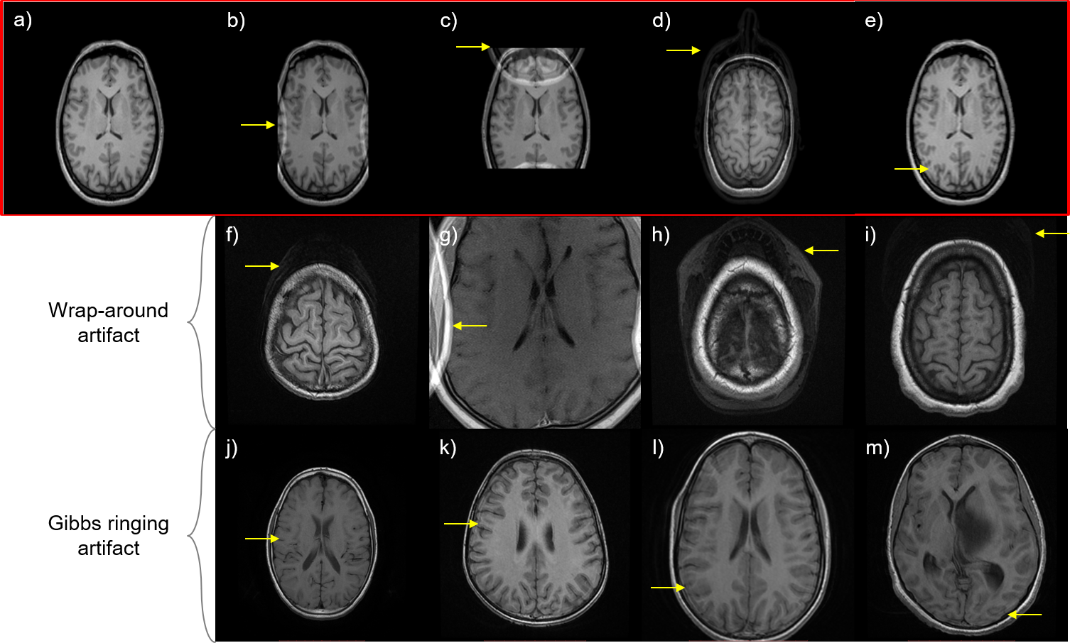
Figure 1. Artifacts simulated in this work and identified in the low-field dataset. a) Representative input brain slice (b-e) Gibbs ringing and wrap-around artifacts simulated in this work b) Gibbs ringing artifact c) X-axis wrap-around artifact d) Y-axis wrap-around artifact e) Z-axis wrap-around artifact (f-i) Wrap-around artifacts identified in the low-field dataset (j-m) Gibbs ringing artifact identified in the low-field dataset.
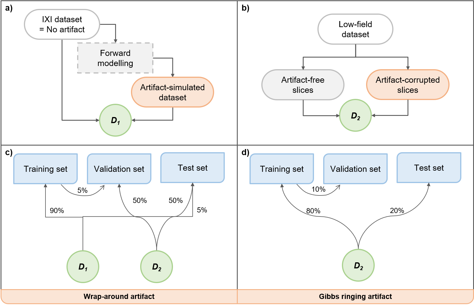
Figure 2. Dataset splits employed in this work. (a-b) Definition of datasets D1 and D2. The publicly available IXI dataset (assumed to be artifact-free) was utilized to obtain the artifact-simulated dataset via forward modelling. These two were combined to obtain dataset D1. In the case of the low-field dataset, artifact-free and artifact-corrupted slices were manually chosen to constitute the dataset D2. (c-d) Training, validation and test set splits derived from datasets D1 and D2.
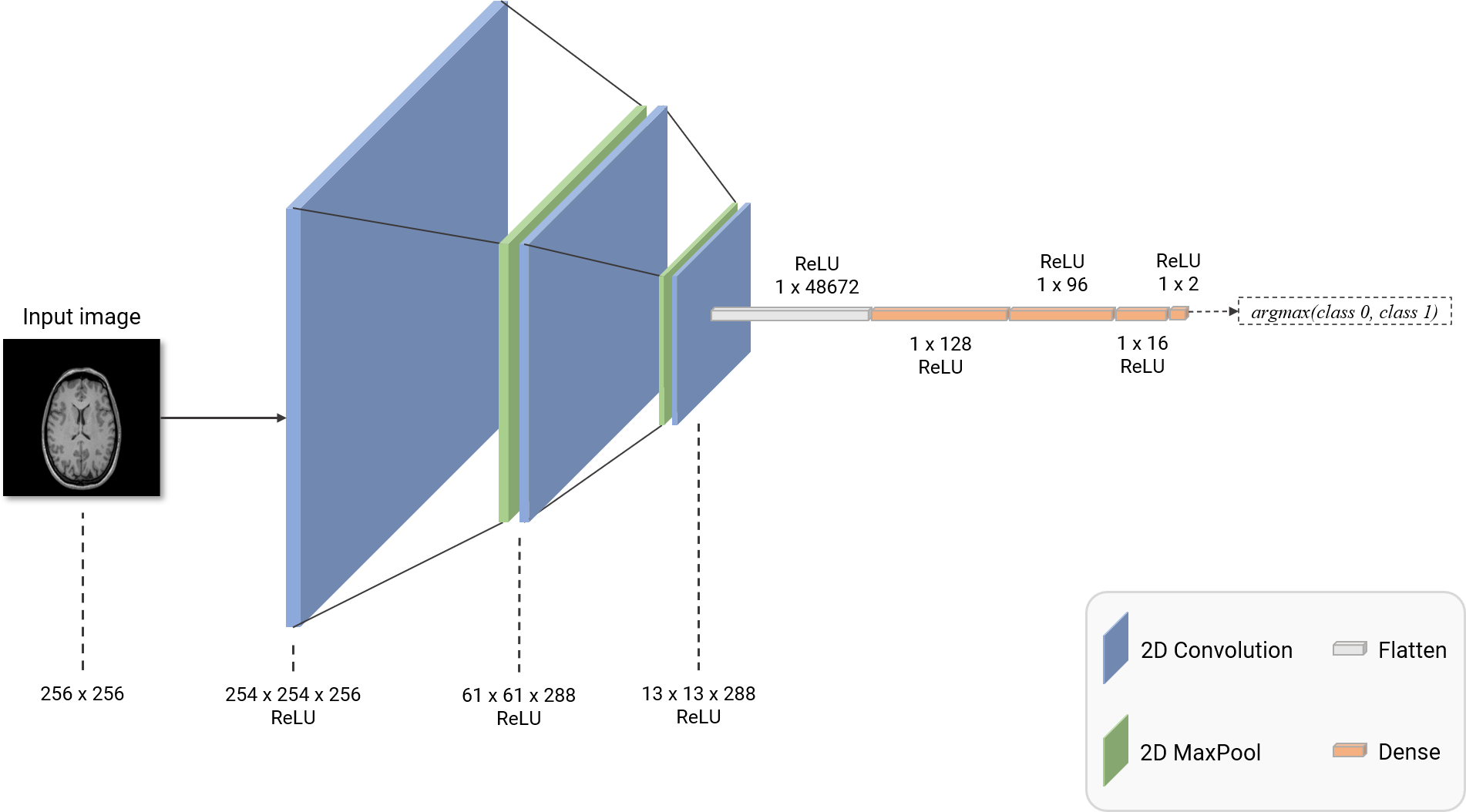
Figure 3. 2D CNN network architecture employed in this work. The 2D convolutional network used in this work constituted three 2D convolution layers (shown in blue) to extract image features and three fully-connected layers (shown in orange) to perform the classification task. Two 2D maxpooling layers were also included, as shown in green. The ‘Flatten’ layer was used to reshape 2D convolutional outputs into a fully-connected layer-compatible 1D vector. Finally, for identifying the artifact, the output was obtained from a ReLU-activated fully-connected layer with two nodes.
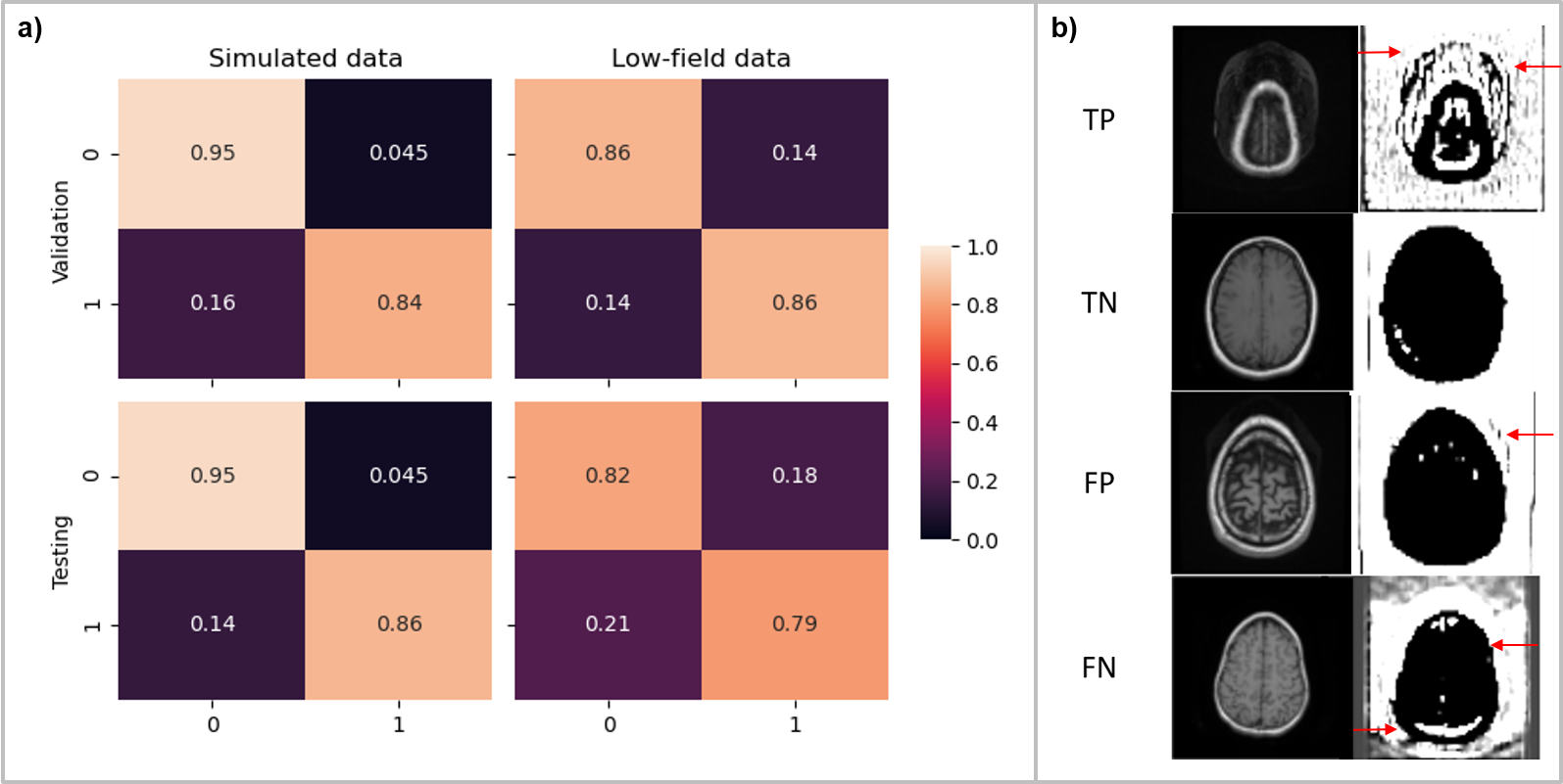
Figure 4. Performance evaluation and model explanation via filter visualization for wrap-around artifact identification. (a) Confusion matrix obtained from the validation and test sets; in the case of simulated data, forward modeling parameters were tweaked based on the validation set results to improve performance. (b) Visualization of representative filters for a true-positive (TP), true-negative (TN), false-positive (FP) and a false-negative (FN) input for explainability.
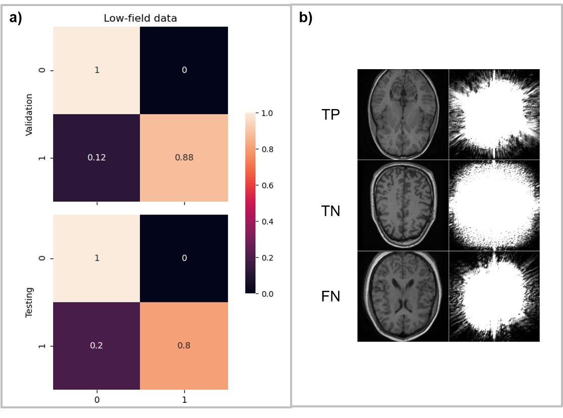
Figure 5. Performance evaluation and model explanation via filter visualization for Gibbs ringing artifact identification. (a) Confusion matrix obtained from the validation and test sets (b) Visualization of representative filters for a true-positive (TP), true-negative (TN) and a false-negative (FN) input for explainability. There were zero FP classification errors across the validation and test sets in this artifact identification task.