Introduction

MRzero is a supervised learning approach for inventing sequences from scratch without providing sequence-programming rules.¹ In previous approaches,^1-3 optimization of sequence parameters and neural networks was performed by using time-consuming average-isochromat-based Bloch simulations. In the present work, fast training of sequence parameters and neural network reconstruction can be achieved by using analytic signal equations as forward model. By performing a joint optimization of both, sequence and neural network parameters, an auto-encoder for simultaneous B1 and T1 mapping is developed and its functionality is tested in vivo at 3T.

Methods

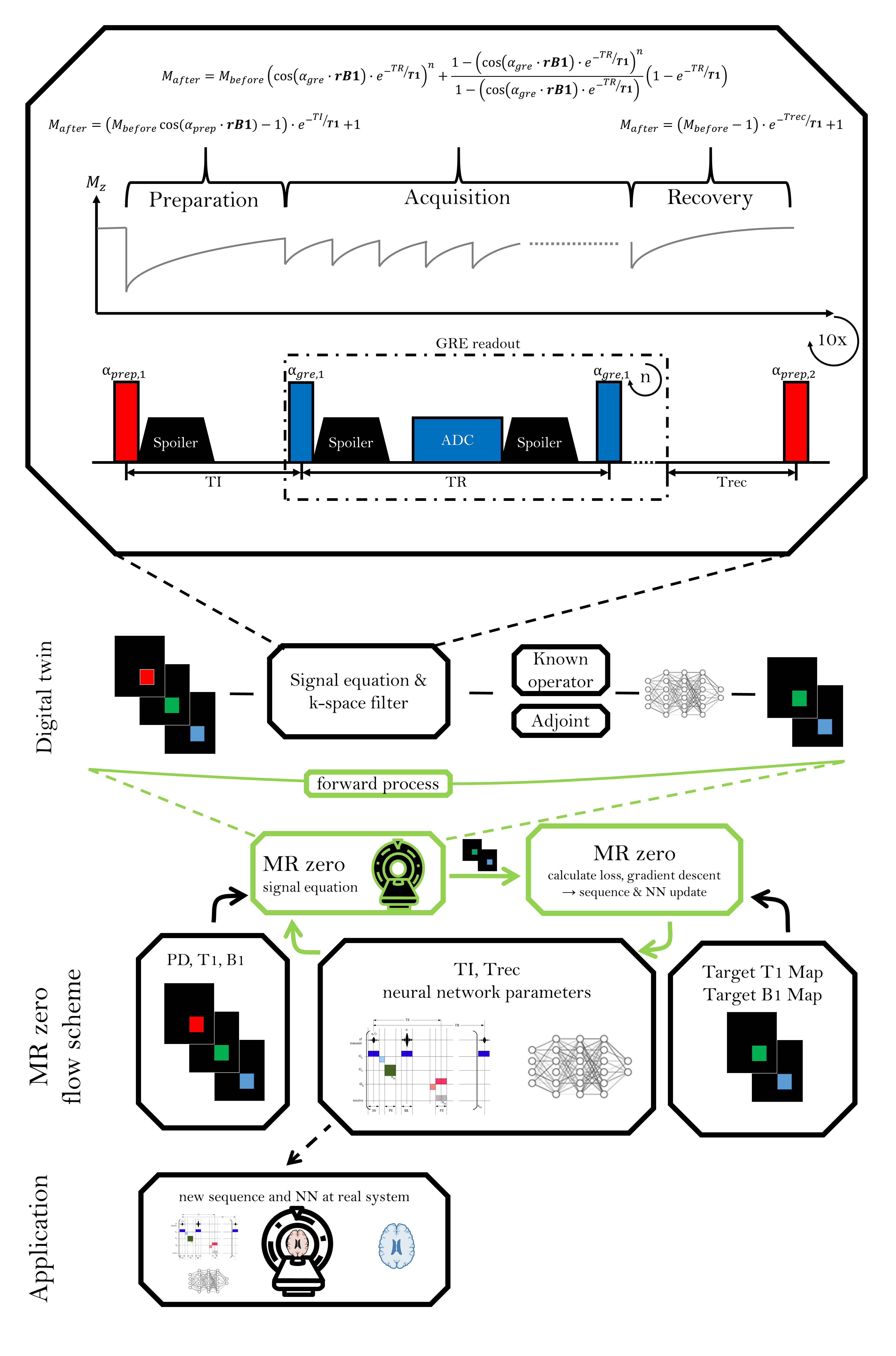
As a basic sequence, 10 subsequent 2D GRE readouts are used (FOV=200mm x 200mm, matrix size 92x92, TR=14ms and $$$\alpha_{gre}$$$=5°). Before each 2D acquisition, a recovery time Trec and a preparation pulse with subsequent delay (TI) is played out for B1 and T1 preparation. A fully connected neural network with three-hidden layers, which maps to B1 and T1, processes the resulting signals. This basic sequence driven as fully relaxed inversion recovery sequence is used as reference for B1 and T1 mapping.
To generate B1 and T1 mapping the complete pipeline (see Figure 1) is used as one function: NN parameters are optimized simultaneously with sequence parameters Trec, TI and $$$\alpha_{prep}$$$, as well as readout parameters TR and $$$\alpha_{gre}$$$. A time and flip angle penalty is applied to enforce shorter sequences with reduced energy deposition.
In contrast to previous work with average-isochromat-based Bloch simulation, an iterative analytic signal equation is used to generate weighted image at every repetition (Figure 1). Each loop consisted of an acquisition, recovery and preparation stage. Longitudinal magnetization after the acquisition of n k-space lines can be described by the geometric series. For the recovery and preparation stages, exponential T1-relaxation is assumed, where the preparation step additionally includes arbitrary initial values accounting for the preparation pulse.
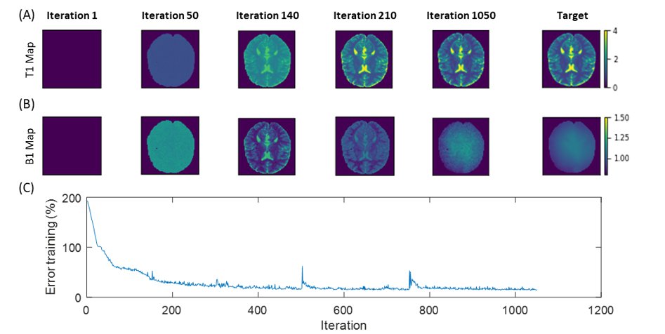
The fully differentiable MRI pipeline is simulated with analytical signal equations with Bloch parameters (PD, B1 and T1) and sequence parameters as input and B1 and T1 as target. Training data consists of square blocks with random size between 16x16 and 64x64, containing random PD, B1 and T1 values, which are passed to the signal equation. As target, these ground truth B1 and T1 values are used. For each optimization iteration, new random B1 and T1 targets are generated at randomly shifted spatial locations. As validation set a numerical brain phantom is used (Figure 2).
The sequences were measured in vivo performed on a PRISMA 3T scanner (Siemens Healthineers, Erlangen Germany) using a 20 channel head coil. Additionally, a B1 map from a WASABI measurement was acquired for comparison.⁴

Results

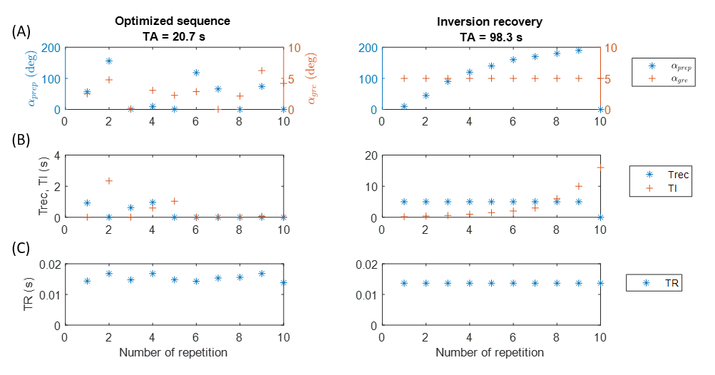
Using the analytical signal equation instead of extensive Bloch simulations, the training time can be reduced by a factor in the range of 2 to 3 orders of magnitude. This results in a total training time for a sequence and NN of less than 9 hours for a resolution of 92x92 trained on CPU.
Figure 3 shows the parameters of the optimized sequence, compared to the fully relaxed inversion recovery sequence. Optimized TRs are in the range of the original inversion recovery sequence. TI and Trec are in the same range from 0s to 2.6s, respectively, but lower on average. Still, acquisition time is reduced from 98.3s to 20.7s. Energy deposition could be roughly decreased by 50% compared to the inversion recovery sequence.
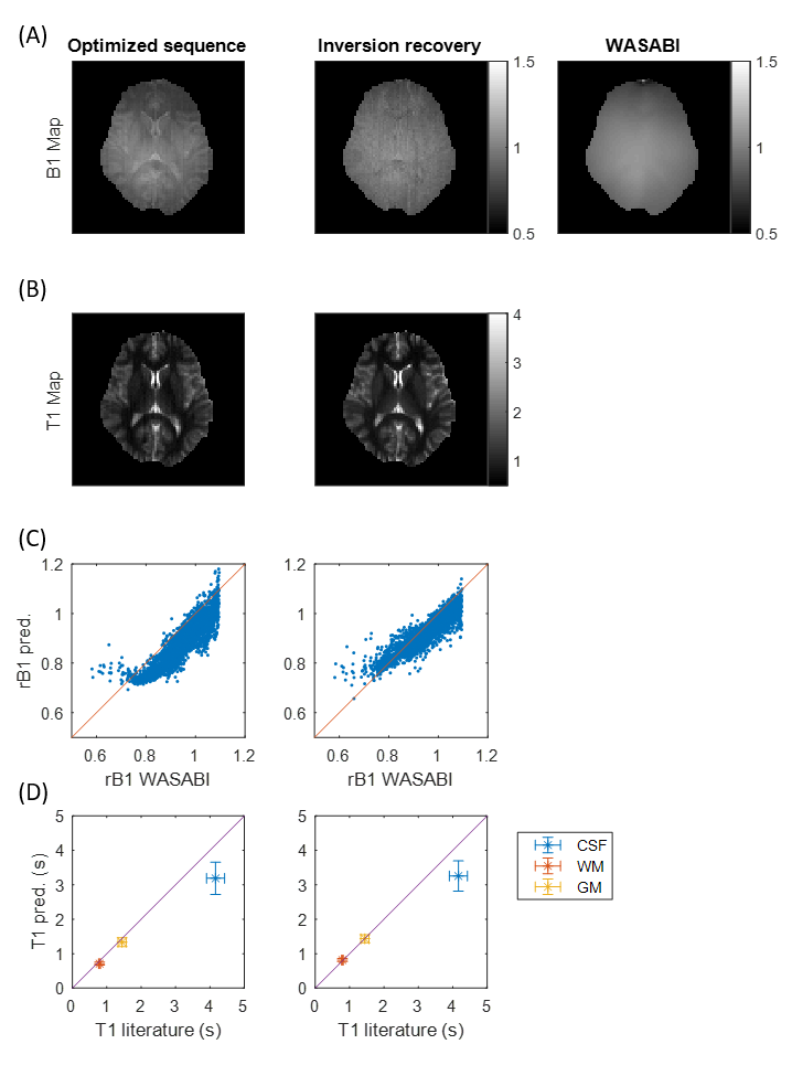
Measured B1 and T1 maps at 3T for a healthy subject are displayed in Figure 4 for the final optimized sequence and the inversion recovery sequence. The acquired B1 maps match well regarding low spatial frequencies to the WASABI B1 map (correlation coefficient R=0.88 between WASABI and optimized sequence and R=0.90 between WASABI and inversion recovery, Figure 4C). Nevertheless, it still shows high spatial frequency artifacts reflecting T1 contrast for the optimized sequence. The obtained T1 map of the optimized sequence matches well to the inversion recovery T1 map and to the literature values at 3T (Figure 4D).⁵ Only in CSF, T1 values are too low, which can be explained by partial volume effects.

Discussion

Simultaneous sequence optimization and NN training was performed solely on synthetic data, but inference on in vivo data provided high quality B1 and T1 maps. The complete training was performed with analytic signal equations, which decreased the computation time drastically by 2 to 3 orders of magnitude. Additionally, without significant loss of information the total acquisition time and the energy deposition could be decreased by 80% and 50%, respectively. Until now only B1 and T1 mapping were shown, but further extension might allow full quantification leading to a self-learning MR fingerprinting⁶ as previously postulated by Zhu et al.⁷
Extending the signal equation by T2, T2* or magnetization transfer would be a next logical step and could solve the B1 deviations in vivo.

Conclusion

We extended the supervised learning-based MR sequence generation framework MRzero by using analytic signal equations as forward model as input for subsequent neural network reconstruction. By performing a joint optimization of both, sequence and neural network parameters, an auto-encoder for simultaneous B1 and T1 mapping was developed and its functionality was confirmed in vivo at 3T. This paves the way to further self-learning MRI pipelines.

Acknowledgements

No acknowledgement found.