1760
Intelligent Incorporation of AI with Model Constraints for MRI Acceleration
Renkuan Zhai1, Xiaoqian Huang2, Yawei Zhao1, Meiling Ji1, Xuyang Lv2, Mengyao Qian1, Shu Liao2, and Guobin Li1
1United Imaging Healthcare, Shanghai, China, 2United Imaging Intelligence, Shanghai, China
1United Imaging Healthcare, Shanghai, China, 2United Imaging Intelligence, Shanghai, China
Synopsis
The advantages of Convolutional Neural Networks (CNN) for MRI acceleration have been widely reported, but one remaining problem is that the significantly complex network makes itself less explainable than conventional model-based methods. In this work, a novel deep learning assisted MRI acceleration method is introduced to address the uncertainty of CNN by integrating its output as another constraint into the framework of Compressed Sensing (CS).
Introduction
Convolutional Neural Networks (CNN)1, an architecture widely used in the field of Artificial Intelligence (AI), has been recently demonstrated to have the potential to outperform conventional image processing methods. Many researches reported superior image reconstruction quality of CNN related methods (e.g. VN 2, U-Net 3) for MRI acceleration. However, as the CNN network is a complicated black box, all related methods are facing a predicament of ensuring their performance and reliability which is critical in clinical scenarios 4. Although larger amount of training data can be helpful for improving stability, the uncertainty could not be addressed as strictly as methods based on mathematical models. Compressed Sensing (CS)5 uses the characteristics of sparse transform to recover information from partially acquired data, however it is difficult to reconstruct tiny anatomic structures perfectly without any prior knowledge. In this study, a novel acceleration framework, AI-assisted Compressed Sensing (ACS), is introduced. By incorporating AI as a regularization term, ACS maintains the advantages of AI while also mathematically addressing the uncertainty of AI.Method
In Compressed Sensing, the reconstruction procedure can be formulated as a minimization problem$$argmin_{x}\|\mathbf{E}x-y\|_2^2+\lambda\|\Phi{x}\|_{1}$$Here, $$$x$$$ denotes the image to be reconstructed. $$$\mathbf{E}$$$ denotes the production of Fourier encoding with binary k-space sampling mask. $$$y$$$ represents the acquired k-space data. $$$\Phi$$$ denotes the sparse transform, e.g. wavelet or total variation.
The key of CS is to find a proper sparse transform to recover information by promoting sparsity, however this is usually not guaranteed in reality due to mismatch between actual anatomic structures and chosen sparse transform. Given $$$x_{AI}$$$ the reconstructed image of the trained AI Module with under-sampled k-space as input and based on the assumption that the predicted image $$$x_{AI}$$$ is close to the true image $$$x$$$, the subtraction operation $$$x-x_{AI}$$$ can actually be taken as a sparse transform. In the spirit of compressed sensing, any significant errors in $$$x_{AI}$$$ due to imperfection in AI Module can be corrected through the use of L1-norm constraint $$$ \|x-x_{AI}\|_{1}$$$. Therefore, by adding one more regularization term from AI Module, formula above can be extended as
$$argmin_{x}\|\mathbf{E}x-y\|_2^2+\lambda_1\|\Phi{x}\|_{1}+\lambda_2\|x-x_{AI}\|_{1}$$Compared to conventional compressed sensing, the introduction of L1 regularization term $$$ \|x-x_{AI}\|_{1}$$$ incorporates the information obtained from the AI Module into iterative reconstruction procedure, which is able to inherit the advantage of AI prediction as well as correct its errors.
Figure 1 shows the flowchart of ACS. Under-sampled k-space data with incoherent trajectories was input to AI Module, which was trained with millions of data with under-sampled k-space as input and corresponding fully-sampled data as ground truth, to generate predicted image $$$x_{AI}$$$. In the final CS Module, both the $$$x_{AI}$$$ and k-space data $$$y$$$ will participate in the iterative reconstruction to produce the final image by solving the function defined in the second formula above.
To evaluate the performance of ACS, images reconstructed with ACS and CS under different acceleration levels were compared. Moreover, to validate the capability of ACS in correcting errors from AI output, artifacts (Gaussian shaped dots) were manually created and inserted into the output from the AI Module in the simulation test.
Volunteer data were acquired on a 3T clinical MR scanner (uMR 780, United Imaging Healthcare, Shanghai, China) with following parameters: T2 FSE 2D of knee with k-space matrix size of [320x288], TR/TE = 3000ms/50ms, echo train length = 11; T2 FSE 2D hip with k-space matrix size of [320x235], TR/TE = 4000ms/120ms, echo train length = 39.
Results & Discussion
Fully-sampled data were used as golden standard. Under-sampled data with net acceleration factor from 2.00x to 4.00x were generated from this fully-sampled data and reconstructed using ACS as well as CS. Results are displayed in Figure 2. ACS showed better performance than CS especially under high acceleration levels.The simulation test results are shown in Figure 3. Artificial Gaussian-shaped artifacts were added to the output of AI Module as shown in Figure 3(b). ACS was able to correct the artifacts from the AI output, as shown in Figure 3(c), and demonstrated good consistency as compared to the fully-sampled golden standard in Figure 3(d).
Conclusion
In conclusion, ACS benefits from AI-provided efficiency and inherits the advantage of CS for information recovery to realize superior MRI acceleration. More importantly, ACS provides a unique way to address the uncertainty of AI by incorporating the output of AI as one more regularization term of conventional compressed sensing.Acknowledgements
No acknowledgement found.References
- Gu J, Wang Z, Kuen J, et al. Recent Advances in Convolutional Neural Networks[J]. Pattern Recognition, 2015.
- Hammernik K, Klatzer T, Kobler E, et al. Learning a variational network for reconstruction of accelerated MRI data[J]. Magnetic Resonance in Medicine, 2017, 79(6).
- Yazdanpanah A P, Afacan O, Warfield S K. Non-learning based deep parallel MRI reconstruction (NLDpMRI)[C]// Image Processing. 2019.
- Antun V, Renna F, Poon C, et al. On instabilities of deep learning in image reconstruction and the potential costs of AI[J]. Proceedings of the National Academy of Sciences, 2020:201907377.
- Lustig M, Donoho D, Pauly J M. Sparse MRI: The application of compressed sensing for rapid MR imaging[J]. Magnetic Resonance in Medicine, 2007, 58(6):1182-1195.
Figures

Figure 1. ACS flowchart: AI Module represents
the trained AI network; CS Module is for solving the second formula using iterative
reconstruction.
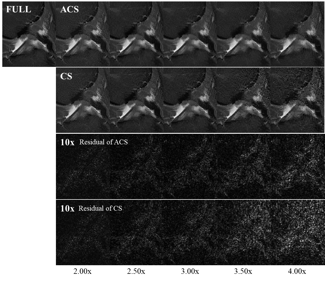
Figure 2. T2 FSE 2D of knee with acceleration factors from 2.00x to 4.00x.
As acceleration factor increased, quality of CS images degraded more rapidly than
ACS.
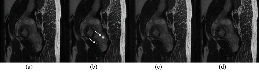
Figure 3. Simulation test results. (a) AI prediction. (b) Artifacts
introduced into the AI prediction manually, as pointed to by the arrows. (c) ACS result.
(d) Fully-sampled original image.