1755

Deep J-Sense: An unrolled network for jointly estimating the image and sensitivity maps

Marius Arvinte¹, Sriram Vishwanath¹, Ahmed H Tewfik¹, and Jonathan I Tamir^1,2,3
¹Electrical and Computer Engineering, The University of Texas at Austin, Austin, TX, United States, ²Diagnostic Medicine, Dell Medical School, The University of Texas at Austin, Austin, TX, United States, ³Oden Institute for Computational Engineering and Sciences, The University of Texas at Austin, Austin, TX, United States

Synopsis

Accurate reconstruction using parallel imaging relies on estimating a set of sensitivity maps from a fully-sampled calibration region, which can lead to reconstruction artifacts in poor signal-to-noise ratio conditions. We introduce Deep J-Sense as a deep learning approach for jointly estimating the image and the sensitivity maps in the frequency-domain. We formulate an alternating minimization problem that uses convolutional neural networks for regularization and train the unrolled model end-to-end. We compare reconstruction performance with model-based deep learning methods that only optimize the image and show that our approach is superior.

Introduction

Combining unrolled iterative optimization with deep learning has greatly improved reconstruction performance in accelerated multi-coil MRI scans when compared to compressed sensing (CS) methods^1,2,3,4. Most approaches rely on estimates of the coil sensitivity maps obtained either through calibration data or via deep neural networks^5,6. When the quality of the estimated sensitivity maps is poor, e.g., low signal-to-noise-ratio (SNR), this can introduce reconstruction artifacts. The need for calibration data also limits the feasible search space for optimal sampling, which could otherwise subsample the center of k-space, making a robust estimator for the sensitivity maps an important practical issue.

In this work, we introduce Deep J-Sense: an approach that jointly estimates the sensitivity maps and the image with the aid of two deep neural networks. Our method combines a model-based approach with deep learning³ to account for the effect of the sensitivity maps in the coil image formation model. We treat the maps as optimization variables and formulate an unrolled alternating minimization problem^7,8, augmented by a denoising convolutional neural network (CNN) for each variable.

We train and evaluate reconstruction performance on the public fastMRI knee dataset⁹. Comparing against MoDL, we demonstrate that our method improves reconstruction performance, increases convergence speed, and accounts for poor SNR conditions.

Theory

J-Sense formalizes image reconstruction as a joint optimization problem and assumes that coil images are formed by pointwise multiplication between an image variable$$$\:\mathbf{x}\:$$$and a set of sensitivity maps$$$\:\mathbf{s}\:$$$^7,8:
$$\min_{\mathbf{x},\mathbf{s}}\lvert\lvert\mathbf{y}-\mathbf{A}(\mathbf{x}\cdot\mathbf{s})\rvert\rvert_2+\lambda_{x}\lvert\lvert\mathbf{x}\rvert\rvert_2+\lambda_{s}\lvert\lvert\mathbf{s}\rvert\rvert_2,$$
where$$$\:\mathbf{A}\:$$$is the forward model incorporating FFT and k-space masking,$$$\:\mathbf{y}\:$$$is the vector of sampled k-space data, and$$$\:\lambda_{x},\lambda{s}\:$$$are regularization coefficients.

We extend the formulation above by defining the variables$$$\:\mathbf{f}=\textrm{IFFT}(\mathbf{x})\:$$$and$$$\:\mathbf{m}=\textrm{IFFT}(\mathbf{s})\:$$$in k-space and replacing the regularization terms with$$$\:\mathcal{N}(f;\mathbf{\theta}_{f})=\lvert\lvert\mathbf{f}-\textrm{FFT}(R_f(\textrm{IFFT}(\mathbf{f});\mathbf{\theta}_f))\rvert\rvert_2\:$$$and$$$\:\mathcal{N}(m;\mathbf{\theta}_{m})=\lvert\lvert\mathbf{m}-\textrm{FFT}(R_m(\textrm{IFFT}(\mathbf{m});\mathbf{\theta}_m))\rvert\rvert_2,\:$$$similar to MoDL³.$$$\:R_f\:$$$and$$$\:R_m\:$$$are learnable CNNs parameterized by weights$$$\:\mathbf{\theta}_{f}\:$$$and$$$\:\mathbf{\theta}_{m},\:$$$respectively. The optimization problem becomes:
$$\min_{\mathbf{f},\mathbf{m}}\lvert\lvert\mathbf{y}-\mathbf{P}(\mathbf{f}\star\mathbf{m})\rvert\rvert_2+\lambda_{f}\mathcal{N}(\mathbf{f};\mathbf{\theta}_f)+\lambda_{m}\mathcal{N}(\mathbf{m};\mathbf{\theta}_m),$$
where$$$\:\mathbf{P}\:$$$is the sampling operator and$$$\:\star\:$$$is a linear convolution. The optimization is unrolled with the iterative steps:

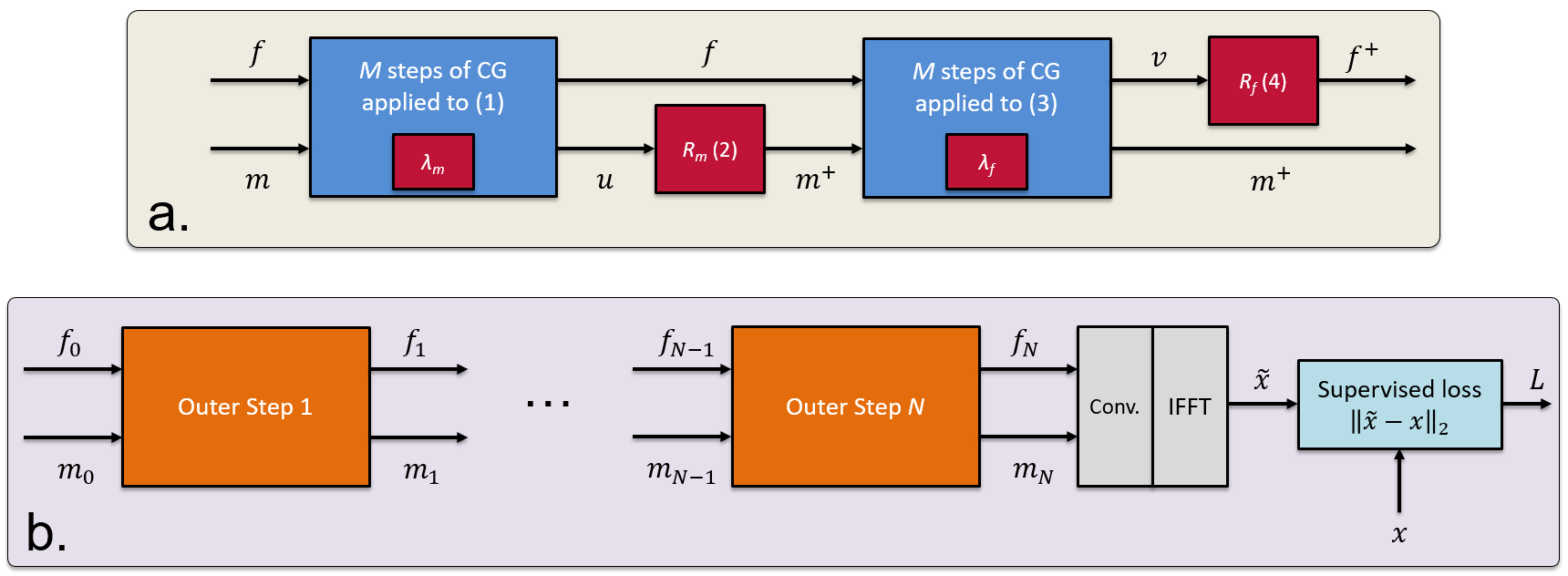
$$$(1)\:\mathbf{u}=\textrm{arg}\min_\mathbf{u}\lvert\lvert\mathbf{y}-\mathbf{A}_{f}\mathbf{u}\rvert\rvert_2+\lambda_m\mathcal{N}(\mathbf{u};\mathbf{\theta}_m)$$$
$$$(2)\:\mathbf{m}=R_m(\mathbf{u};\mathbf{\theta}_m)$$$
$$$(3)\:\mathbf{v}=\textrm{arg}\min_\mathbf{v}\lvert\lvert\mathbf{y}-\mathbf{A}_{m}\mathbf{v}\rvert\rvert_2+\lambda_f\mathcal{N}(\mathbf{v};\mathbf{\theta}_f)$$$
$$$(4)\:\mathbf{f}=R_f(\mathbf{v};\mathbf{\theta}_f)$$$

$$$\mathbf{A}_f\:$$$and$$$\:\mathbf{A}_m\:$$$are forward operators that include linear convolution with$$$\:\mathbf{f}\:$$$or$$$\:\mathbf{m},\:$$$and sampling. Steps (1) and (3) are approximately solved with$$$\:M\:$$$iterations of the Conjugate Gradient (CG) algorithm. Steps (2) and (4) represent a forward pass through a CNN. We treat$$$\:\lambda_f\:$$$and$$$\:\lambda_m\:$$$as learnable parameters. Without steps (1) and (2), our approach becomes a frequency-domain version of MoDL.

Importantly, Deep J-Sense treats both the image and sensitivity maps as frequency domain kernels and assumes a linear convolution model in k-space. To account for the smoothness of the sensitivity maps in the image domain, we restrict the kernel$$$\:\mathbf{m}\:$$$to a small size in k-space. This is different than prior work that optimizes the sensitivity maps directly in the image domain^5,10. To obtain a linear convolution in frequency, the image kernel$$$\:\mathbf{f}\:$$$has size$$$\textrm{dim}(\mathbf{y})+\textrm{dim}(\mathbf{m})-1$$$.

Optimization is initialized with$$$\:(f_0,m_0),\:$$$unrolled for a number of$$$\:N\:$$$times, and the output coils are computed as$$$\:\hat{\mathbf{x}}=\mathbf{f}_N\star\mathbf{m}_N$$$. The two networks and$$$\:\lambda\:$$$coefficients are reused across all unrolls. The parameters$$$\:\mathbf{\theta}_f,\mathbf{\theta}_m,\lambda_f,\lambda_m\:$$$are trained using a supervised loss on the root-sum-square (RSS) images. A block diagram is shown in Fig.1.

Methods

We implement Deep J-Sense using PyTorch. We use a CG algorithm defined over complex variables, and CNNs defined over real variables (with 2x channels). The networks use a ResNet¹¹ architecture with three residual blocks, 64 hidden channels, and ReLU activations. Training data is used from the fastMRI multi-coil kneel dataset. We use five central slices from each scan, for a total of$$$\:4865\:$$$training slices from both fat-suppressed (FS) and non-fat-suppressed (NFS) contrasts. Validation is over$$$\:995\:$$$slices from both contrasts. We train our model with$$$\:(N,M)=(6,3)\:$$$for 20 epochs using the Adam optimizer with batch size$$$\:1,\:$$$learning rate$$$\:10^{-4},\:$$$gradient clipping and progressive unrolling³.

For comparison, we implement MoDL with$$$\:(N,M)=(6,6)\:$$$and$$$\:R_f\:$$$of depth three (MoDL-3) or six (MoDL-6). We train with the same hyper-parameters, same number of epochs, and on the same data. We simulate J-Sense¹² with$$$\:(N,M)=(6,3)\:$$$and$$$\:\lambda_{f}=\lambda_{m}=0.01\:$$$. We use a map kernel of size$$$\:25\times25\:$$$for Deep J-Sense, initialized with an RSS estimate from the undersampled data. For MoDL, we use sensitivity maps estimated with the auto-ESPIRiT^13,14 algorithm using BART¹⁵. For J-Sense, we initialize the maps with zeroes.

Results and Discussion

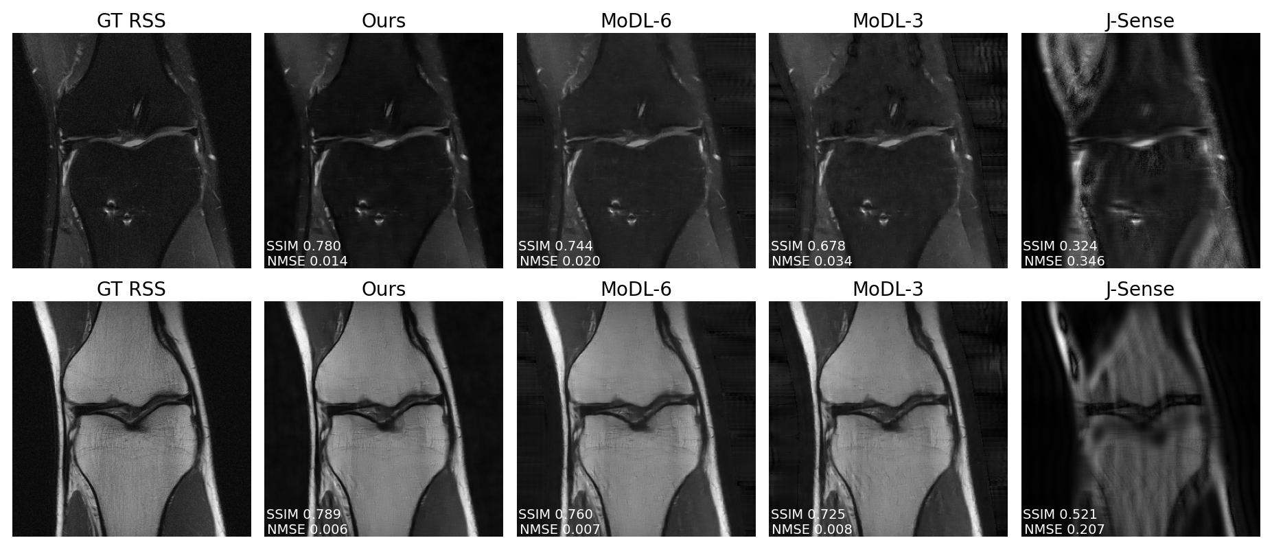
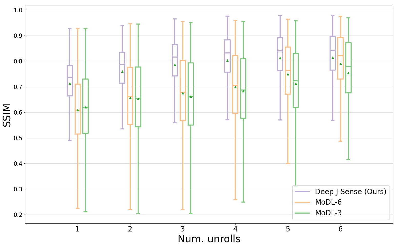
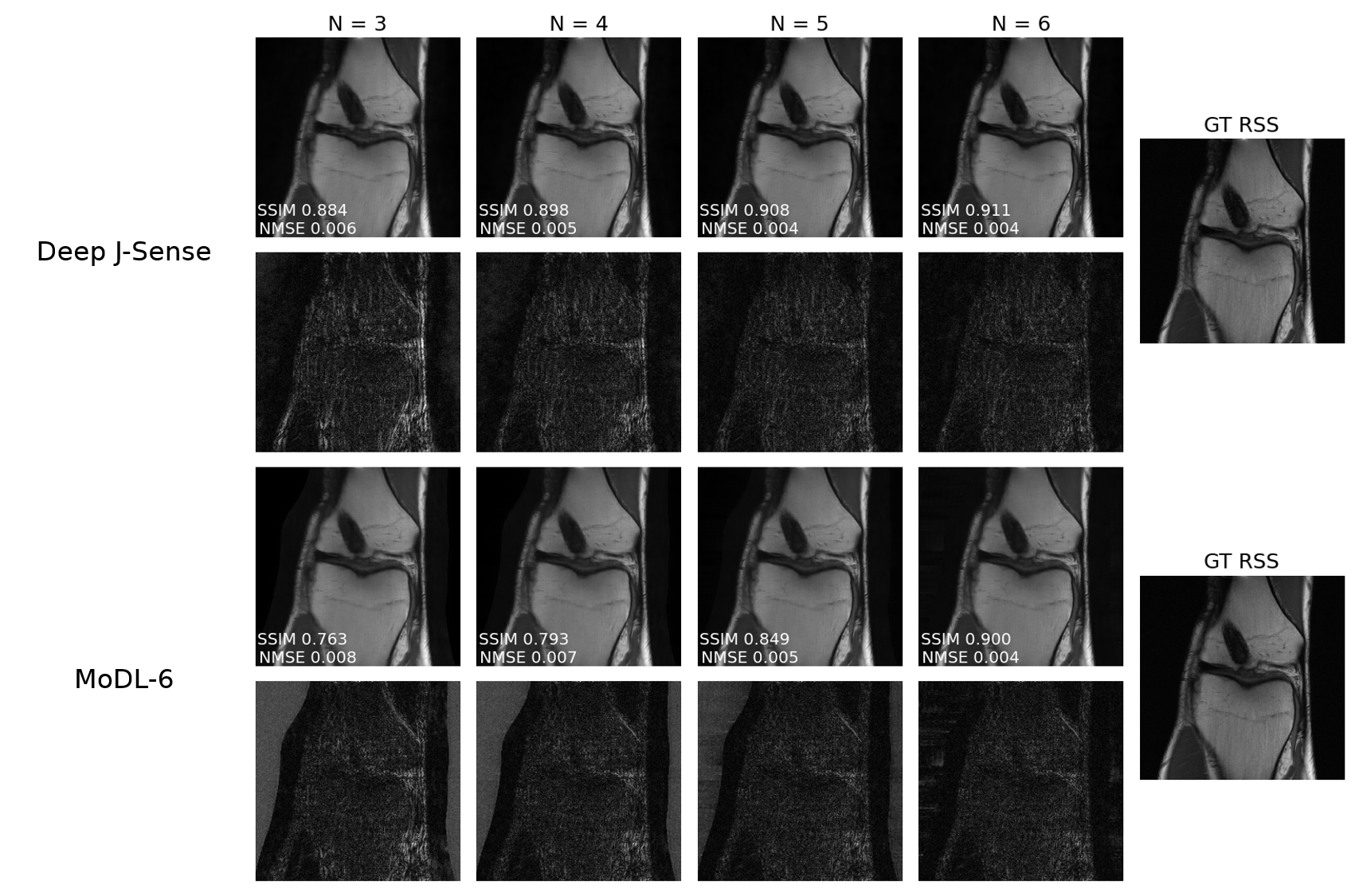
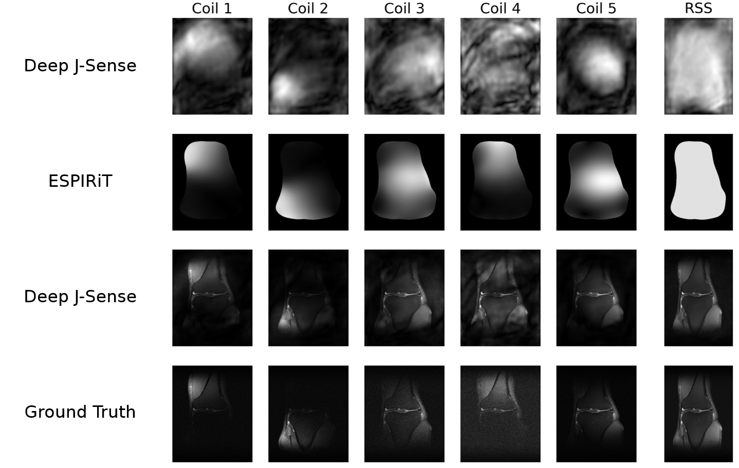
Fig.2 shows example reconstructions on two validation slices at acceleration factor$$$\:R=4\:$$$. Deep J-Sense gives the lowest reconstruction error, followed by MoDL and J-Sense. Because of the limited number of inner CG steps and the random sampling pattern, J-Sense converges to a poor solution, highlighting the role the networks$$$\:R_f\:$$$and$$$\:R_m\:$$$play in stabilizing the alternating optimization. Fig.3 shows the boxplot of the validation structural similarity index (SSIM). Deep J-Sense enjoys faster convergence and outperforms MoDL even when the latter uses a network twice as deep.

Fig.4 plots the intermediate reconstruction results after each unroll for Deep J-Sense and MoDL. The end performance is comparable between the two, but Deep J-Sense converges faster, while MoDL spends iterations correcting errors outside of the region of interest. Fig.5 plots a subset of learned sensitivity maps and reconstructed coil images. Compared to the ESPIRiT estimate, our maps contain higher frequency components. This is likely a consequence of the existence of multiple optimal solution sets of maps that form a clean RSS solution, indicating that the scheme may learn a notion of uncertainty in poor SNR conditions. Although not explored here, the joint-estimation may also support non-autocalibrated sampling schemes.

Conclusion

Sensitivity map estimation can lead to artifacts and slow convergence of unrolled methods. We have introduced a deep learning approach to jointly estimate the maps and image in k-space.

Acknowledgements

This work was supported by the Office of Naval Research grant N00014-19-1-2590.

References

1. Lustig, M., Donoho, D. L., Santos, J. M., & Pauly, J. M. (2008). Compressed sensing MRI. IEEE Signal Processing Magazine, 25(2), 72-82.

2. Hammernik, K., Klatzer, T., Kobler, E., Recht, M. P., Sodickson, D. K., Pock, T., & Knoll, F. (2018). Learning a variational network for reconstruction of accelerated MRI data. Magnetic Resonance in Medicine, 79(6), 3055-3071.

3. Aggarwal, H. K., Mani, M. P., & Jacob, M. (2018). MoDL: Model-based deep learning architecture for inverse problems. IEEE Transactions on Medical Imaging, 38(2), 394-405.

4. Recht, M.P., Zbontar, J., Sodickson, D.K., Knoll, F., Yakubova, N., Sriram, A., Murrell, T., Defazio, A., Rabbat, M., Rybak, L. & Kline, M., 2020. Using Deep Learning to Accelerate Knee MRI at 3 T: Results of an Interchangeability Study. American Journal of Roentgenology, 215(6), 1421-1429.

5. Sriram, A., Zbontar, J., Murrell, T., Defazio, A., Zitnick, C.L., Yakubova, N., Knoll, F. & Johnson, P., 2020. End-to-End Variational Networks for Accelerated MRI Reconstruction. arXiv preprint arXiv:2004.06688.

6. Peng, X., Perkins, K.,Clifford, B., Sutton, B., & Liang Z.-P., 2018. Deep-SENSE: Learning Coil Sensitivity Functions for SENSE Reconstruction Using Deep Learning. Proc. ISMRM 2018, Paris.

7. Ying, L., & Sheng, J. (2007). Joint image reconstruction and sensitivity estimation in SENSE (JSENSE). Magnetic Resonance in Medicine: An Official Journal of the International Society for Magnetic Resonance in Medicine, 57(6), 1196-1202.

8. Uecker, M., Hohage, T., Block, K. T., & Frahm, J. (2008). Image reconstruction by regularized nonlinear inversion—joint estimation of coil sensitivities and image content. Magnetic Resonance in Medicine, 60(3), 674-682.

9. Zbontar, J., Knoll, F., Sriram, A., Murrell, T., Huang, Z., Muckley, M.J., Defazio, A., Stern, R., Johnson, P., Bruno, M., & Parente, M., 2018. fastMRI: An open dataset and benchmarks for accelerated MRI. arXiv preprint arXiv:1811.08839.

10. Jun, Y., Shin, H., & Eo, T., 2020. Joint-ICNet: Joint Deep Model-based MR Image and Coil Sensitivity Reconstruction Network for Fast MRI. fastMRI 2020 Competition Leaderboards, https://fastmri.org/leaderboards/challenge/.

11. He, K., Zhang, X., Ren, S., & Sun, J. (2016). Deep residual learning for image recognition. In Proceedings of the IEEE Conference on Computer Vision and Pattern Recognition (pp. 770-778).

12. Ong, F., & Lustig, M. (2019, May). SigPy: a python package for high performance iterative reconstruction. In Proceedings of the ISMRM 27th Annual Meeting, Montreal, Quebec, Canada (Vol. 4819).

13. Uecker, M., Lai, P., Murphy, M.J., Virtue, P., Elad, M., Pauly, J.M., Vasanawala, S.S., & Lustig, M., 2014. ESPIRiT—an eigenvalue approach to autocalibrating parallel MRI: where SENSE meets GRAPPA. Magnetic Resonance in Medicine, 71(3), pp.990-1001.

14. Iyer, S., Ong, F., Setsompop, K., Doneva, M., & Lustig, M., 2020. SURE‐based automatic parameter selection For ESPIRiT calibration. Magnetic Resonance in Medicine, 84(6), pp.3423-3437.

15. Uecker, M., Ong, F., Tamir, J. I, Bahri D., Virtue P., Cheng JY, Zhang T., & Lustig M., 2015. Berkeley Advanced Reconstruction Toolbox. Proc ISMRM 2015, Toronto

Figures

Block diagram of the approach. (a) Inside each unrolling step, the pair of variables is updated in an alternating fashion with M steps of CG applied to each variable. The red blocks represent the learnable parameters of Deep J-Sense and are shared across unrolls. The numbers in parentheses corresponding to the four update steps in the text. (b) N unrolls are applied starting from initial values. At each step, the gradient of the loss term is back-propagated to the trainable parameters and an update is performed.

Reconstruction comparison with R = 4 for two validation slices. Top row: FS scan. Bottom row: NFS scan. In order, from left to right: ground truth RSS image, Deep J-Sense (three residual blocks for each variable), MoDL-6 (six residual blocks), MoDL-3 (three residual blocks) and J-Sense. All results are obtained with N = 6 unrolls. SSIM and NSME values are indicated in the bottom-left corner of each image.

Statistical results for reconstruction performance on the fastMRI knee validation set (995 slices) with R = 4. All methods are trained with N = 6 unrolls and tested at various CNN depths indicated on the x-axis. The y-axis indicates the SSIM value. Solid triangles and solid lines represent the mean and median values, respectively.

Reconstruction results for R = 4 after each outer loop unroll (starting from three) for a validation slice. The first row and third rows represent the estimated RSS images for Deep J-Sense and MoDL-6, respectively. The second and fourth rows represent the pixel-wise error for Deep J-Sense and MoDL-6, respectively. Both methods perform similarly after six unrolls, but the proposed approach converges faster and is more stable. The convergence of MoDL is affected by peripheral regions with near-zero signal values.

Examples of estimated sensitivity maps and reconstructed coil images output by our method after N = 6 unrolls for a validation sample with R = 4. The first five columns show specific coils and the last columns shows the RSS image obtained from all 15 coils. The first row shows the estimated sensitivity maps, obtained by zero-padding and IFFT of the estimated frequency-domain kernel. The second row shows the sensitivity maps estimated using the auto-ESPIRiT algorithm. The third row shows the reconstructed coil images. The fourth row shows the ground truth (fully-sampled) coil images.

Proc. Intl. Soc. Mag. Reson. Med. 29 (2021)

1755