1726
Subsampling an existing diffusion MRI multi-shell scheme: impact on histogram measures derived from DTI and DKI1ISR-Lisboa/LARSyS and Department of Bioengineering, Instituto Superior Técnico, Universidade de Lisboa, Lisbon, Portugal, 2Neurology Department, Hospital da Luz, Lisbon, Portugal, 3Learning Health, Hospital da Luz, Lisbon, Portugal
Synopsis
Multi-shell diffusion MRI sampling schemes require long acquisition times and are hence potentially compromised by poorer subject compliance. There is therefore a need to consider strategies to enable shortening the exam to ensure clinical feasibility, while maintaining cross-exam comparability. We analyzed the impact of subsampling a multi-shell scheme on the estimation of diffusion maps. In particular, we evaluated its effect on histogram-derived metrics computed over skeletonized maps of DTI and DKI parameters. Several metrics showed a significant effect of subsampling. This should be carefully considered depending on the effect size we are trying to measure on a patient’s population.
Introduction
Diffusion MRI (dMRI) is a commonly used technique to obtain sensitive biomarkers of brain pathology. Diffusion-tensor imaging1(DTI) is still the most used signal model in clinical routine, where single-shell acquisitions are usually performed due to time limitations. To improve specificity, more complex signal models such as diffusion kurtosis (DKI)2 can be used, which however require multi-shell acquisition schemes (with multiple b-values and a higher number of gradient directions) with inevitably longer acquisition times. In clinical studies with strict time constraints and potentially poor patient compliance (specially multi-session studies)3, it is likely that the acquisition may need to be shortened a priori, or interrupted before completion. To ensure clinical feasibility and cross-exam comparability, there is hence a need to design dMRI studies considering more efficient sampling strategies, whether by reordering spatially close gradient directions4 and/or decreasing the total number of gradient directions per shell5,6. Here, we analyzed the impact of subsampling a multi-shell dMRI acquisition scheme on the estimation of diffusion parameter maps based on DTI (FA, MD, AD and RD) and DKI (MK, AK, and RK). In particular, we evaluated its impact on histogram measures computed over skeletonized diffusion maps.Methods
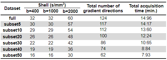
Data acquisition:We acquired 9 dMRI datasets using a DWI-EPI sequence on a 3T Siemens Vida system with a 64-channel RF-receive head coil with the following parameters: TR/TE=6800/89ms, 66 slices, in-plane GRAPPA factor 2, SMS factor 3, 2mm isotropic resolution. The sampling scheme consisted of 3 diffusion shells with b=400,1000,2000s/mm2 along 32,32,60 gradient directions, respectively; and 8 non-diffusion-weighted volumes.
Subsampling and data processing:
Firstly, we generated 6 optimal subsets by uniformly discarding7 5, 10, 20, 30, 40 or 50% of the total number of directions per shell (Table 1), using MATLAB (mathworks.com). Data preprocessing was carried out following the DESIGNER pipeline8: denoising and Gibbs ringing correction9 with MRTrix (mrtrix.org/); Rician bias correction10 geometric, eddy-current distortions and motion correction11-13 with FSL (fsl.fmrib.ox.ac.uk/fsl), and bias field correction with MRTrix. Tensor-fitting was performed based on b=1000,2000s/mm2 shells with dkimodel.fit function from DIPY (dipy.org) to derive maps of: FA, MD, AD, RD, MK, AK and RK. Skeletonised maps were generated using FSL’s tract-based spatial statistics (TBSS)14. A mean FA skeleton was obtained considering the fully sampled dataset and its subsets.
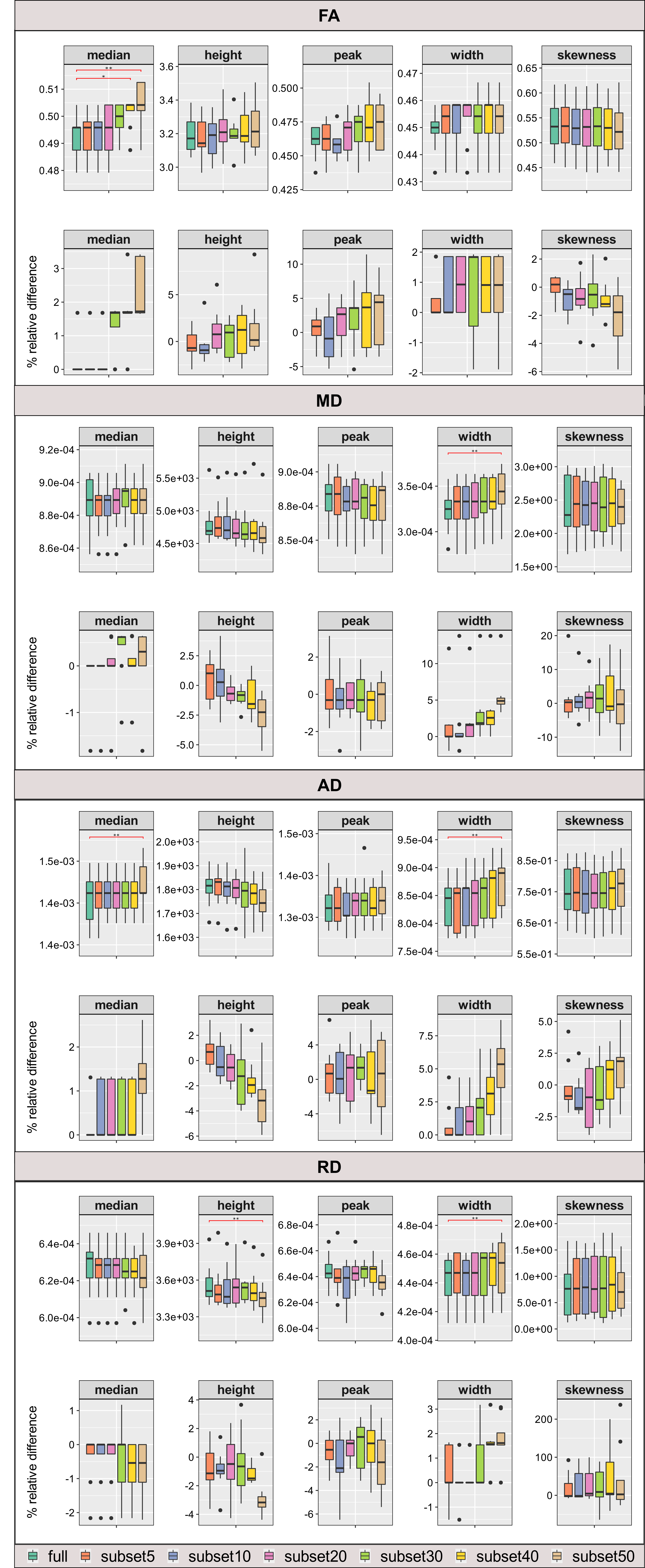
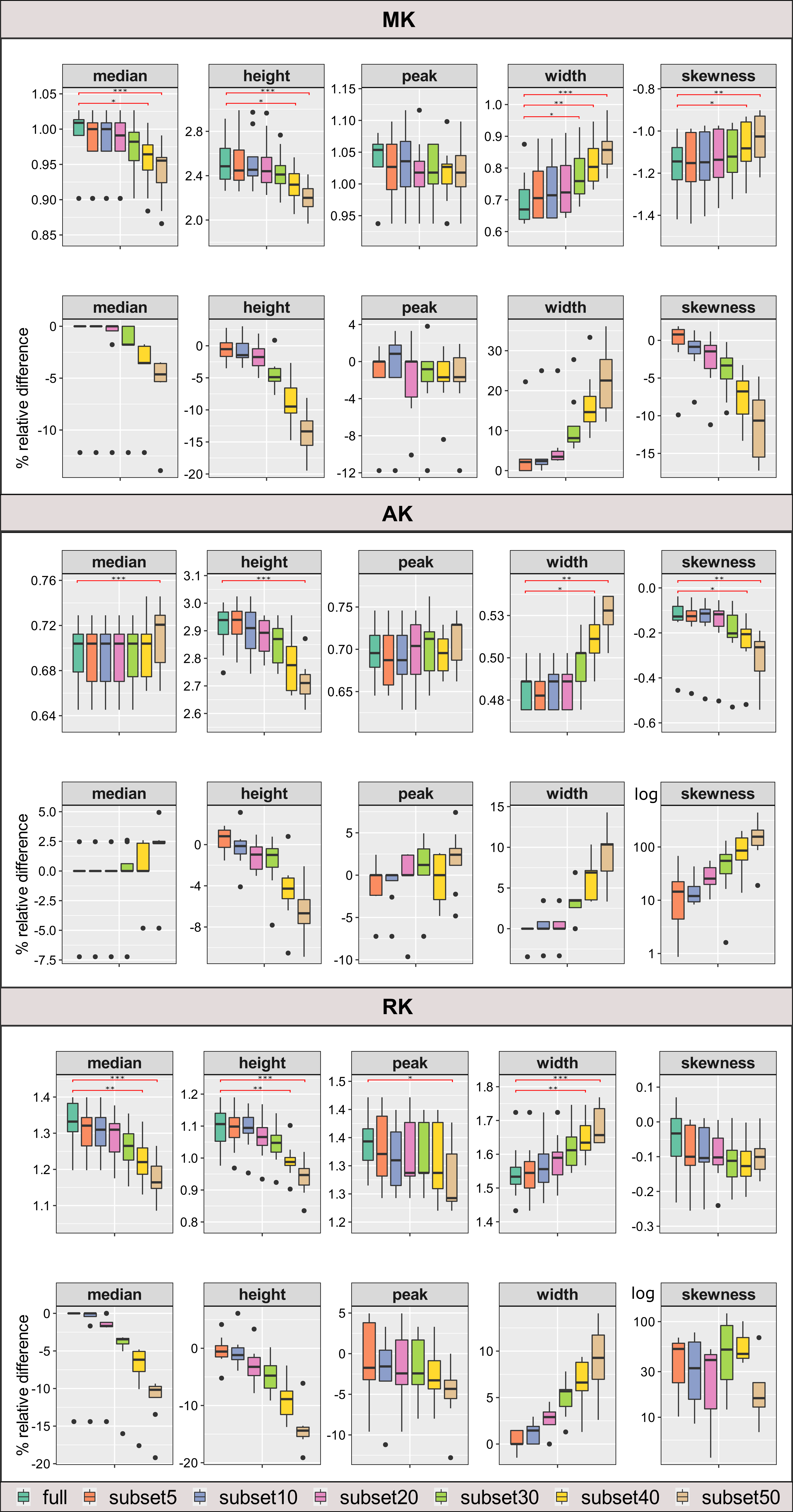
To analyze the effects of subsampling, histograms of each diffusion parameter were computed across on the respective skeletonised maps, using R (r-project.org/)(optimal number of bins estimated with Freedman-Diaconis'15 rule), for each full dataset and corresponding subsets. Then, the following histogram-based metrics were extracted for each parameter and dataset: median, peak height, peak value, width (difference between 95th and 5th percentiles16); and skewness. The metrics obtained for each subset were compared with the ones obtained with the respective full dataset, using the nonparametric Friedman test and Conover’s Test for post-hoc analysis (Bonferroni correction, p<0.05), on JASP (jasp-stats.org/). The associated error was computed as the relative difference (in percentage) between the metric obtained from each subset and the full dataset.
Results/Discussion
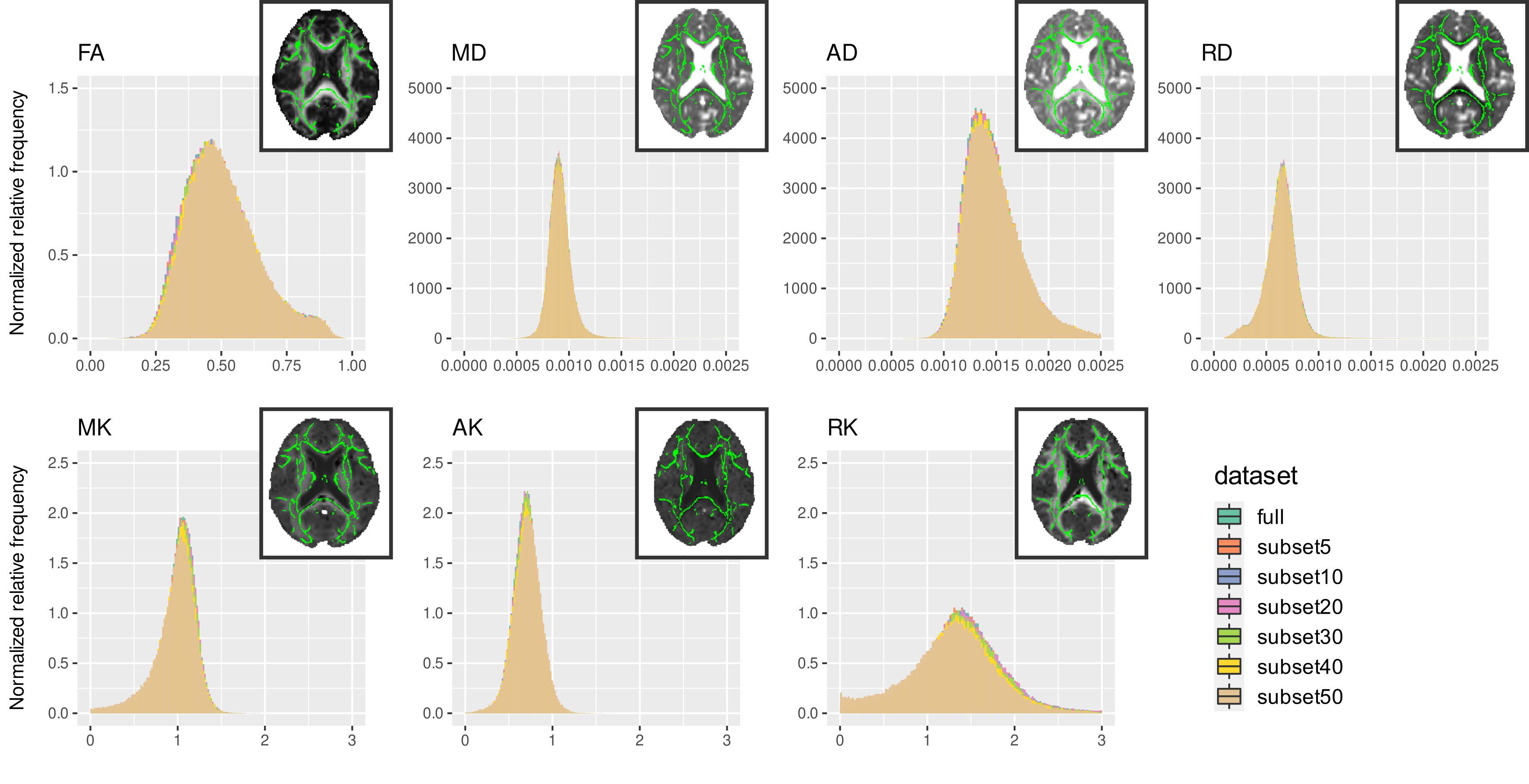
Figure 1 illustrates the histograms of skeletonised DTI and DKI parameter maps. The distributions of histogram metrics are shown for DTI parameters (Figure 2) and DKI parameters (Figure 3), for both the full dataset and the subsets, together with the respective relative difference with respect to the full dataset. Several histogram metrics of DTI and DKI parameters showed a significant effect of subsampling, with sub-sampled data providing biased estimates of all metrics. Histogram metrics derived for DKI parameters were more prone to undersampling bias than DTI metrics. This effect is expected given that parameter estimation from DKI models is more susceptible to noise17. In particular, the FA median was significantly overestimated for subset40 and subset50 up to a maximum error of 3%. This supports previous reports reporting that for a robust estimation of anisotropy at least 20 unique sampling directions are necessary5. AD was overestimated up to a maximum error of 3%, a finding that is consistent with 18. Moreover, subset50 showed a significantly increased peak width compared to the full dataset for MD, AD and RD, which is representative of more widespread values. On the other hand, MK (subset40 and subset50) and RK (subset40 and subset50) were underestimated by up to 20% and AK (subset40 and subset50) was overestimated by 5%.Conclusion
In scenarios where shortening the protocol is necessary, and to allow reusing existing data, a trade-off between minimizing bias on histogram measures and shortening scan time should be carefully considered depending on the expected effect size on a patient’s population. For example, by shortening the acquisition for 5 minutes (subset30) most of the errors are under 5% for all measures.Acknowledgements
We acknowledge the Portuguese Science Foundation through grants SFRH/BD/139561/2018, PTDC/EMD-EMD/29675/2017, LISBOA-01-0145-FEDER-029675 and UIDB/50009/2020.References
1. Basser PJ, Mattiello J, LeBihan D. MR diffusion tensor spectroscopy and imaging. Biophysical Journal. 1994;66(1):259-267. doi:10.1016/s0006-3495(94)80775-1.
2. Jensen JH, Helpern JA, Ramani A, Lu H, Kaczynski K. Diffusional kurtosis imaging: The quantification of non-gaussian water diffusion by means of magnetic resonance imaging. Magnetic Resonance in Medicine. 2005;53(6):1432-1440. doi:10.1002/mrm.20508.
3. Jelescu IO, Budde MD. Design and validation of diffusion MRI models of white matter. Front Phys. 2017;28. doi:10.3389/fphy.2017.00061.
4. Dubois J, Poupon C, Lethimonnier F, Le Bihan D. Optimized diffusion gradient orientation schemes for corrupted clinical DTI data sets. MAGMA. 2006;19(3):134-143.
5. Jones DK. The effect of gradient sampling schemes on measures derived from diffusion tensor MRI: a Monte Carlo study. Magn Reson Med. 2004;51(4):807-815.
6. Lebel C, Benner T, Beaulieu C. Six is enough? Comparison of diffusion parameters measured using six or more diffusion-encoding gradient directions with deterministic tractography. Magn Reson Med. 2012;68(2):4.74-483.
7. Cheng J, Shen D, Yap P-T. Designing single- and multiple-shell sampling schemes for diffusion MRI using spherical code. Med Image Comput Comput Assist Interv. 2014;17(Pt 3):281-288.
8. Ades-Aron B, Veraart J, Kochunov P, et al. Evaluation of the accuracy and precision of the diffusion parameter EStImation with Gibbs and NoisE removal pipeline. Neuroimage. 2018;183:532-543.
9. Veraart J, Fieremans E, Novikov DS. Diffusion MRI noise mapping using random matrix theory. Magn Reson Med. 2016;76(5):1582-1593.
10. Koay CG and Basser PJ. Analytically exact correction scheme for signal extraction from noisy magnitude MR signals. J Magn Reson. 2006;179(2):317-322.
11. Andersson JLR, Skare S, Ashburner J. How to correct susceptibility distortions in spin-echo echo-planar images: application to diffusion tensor imaging. Neuroimage. 2003;20(2):870-888.
12. Andersson JLR, Sotiropoulos SN. An integrated approach to correction for off-resonance effects and subject movement in diffusion MR imaging. Neuroimage. 2016;125:1063-1078.
13. Andersson JLR, Sotiropoulos SN. Non-parametric representation and prediction of single- and multi-shell diffusion-weighted MRI data using Gaussian processes. Neuroimage. 2015;122:166-176.
14. Smith SM, Jenkinson M, Johansen-Berg H, et al. Tract-based spatial statistics: voxelwise analysis of multi-subject diffusion data. Neuroimage. 2006;31(4):1487-1505.
15. Freedman D, Diaconis P. On the histogram as a density estimator:L 2 theory. Zeitschrift für Wahrscheinlichkeitstheorie und Verwandte Gebiete. 1981;57(4):453-476. doi:10.1007/bf01025868.
16. Baykara E, Gesierich B, Adam R, et al. A Novel Imaging Marker for Small Vessel Disease Based on Skeletonization of White Matter Tracts and Diffusion Histograms. Ann Neurol. 2016;80(4):581-592.
17. Hutchinson EB, Avram AV, Irfanoglu MO, et al. Analysis of the effects of noise, DWI sampling, and value of assumed parameters in diffusion MRI models. Magn Reson Med. 2017;78(5):1767-1780.
18. Pierpaoli C, Basser PJ. Toward a quantitative assessment of diffusion anisotropy. Magnetic Resonance in Medicine. 1996;36(6):893-906. doi:10.1002/mrm.1910360612
Figures