1720
Estimation of individual brain signature and node-wise sensibility by a community-based DW-MRI connectome analysis1Signal Processing Lab (LTS5), École Polytechnique Fédérale de Lausanne, Lausanne, Switzerland, 2Computer Science Department, CIMAT, Centro de Investigación en Matemáticas, Guanajuato, Mexico, 3CIBM Center for BioMedical Imaging, Lausanne, Switzerland, 4Radiology Department, Centre Hospitalier Universitaire Vaudois and University of Lausanne, Lausanne, Switzerland
Synopsis
In this work, we study the effect of the reconstruction pipeline s on the reproducibility and sensitivity of the DW-MRI brain connectivity graphs. The brain database we analyze contains several scan repetitions that allow us to characterize the impact of different reconstruction pipeline parameters on the connectomes' topology. We use a novel methodology to detect robust graph communities and show the level of reproducibility of the brain structure/biomarkers. Moreover, we proposed a tool to identify the less-robust graph nodes that suffer the effects of the reconstruction pipelines' variability.
Introduction
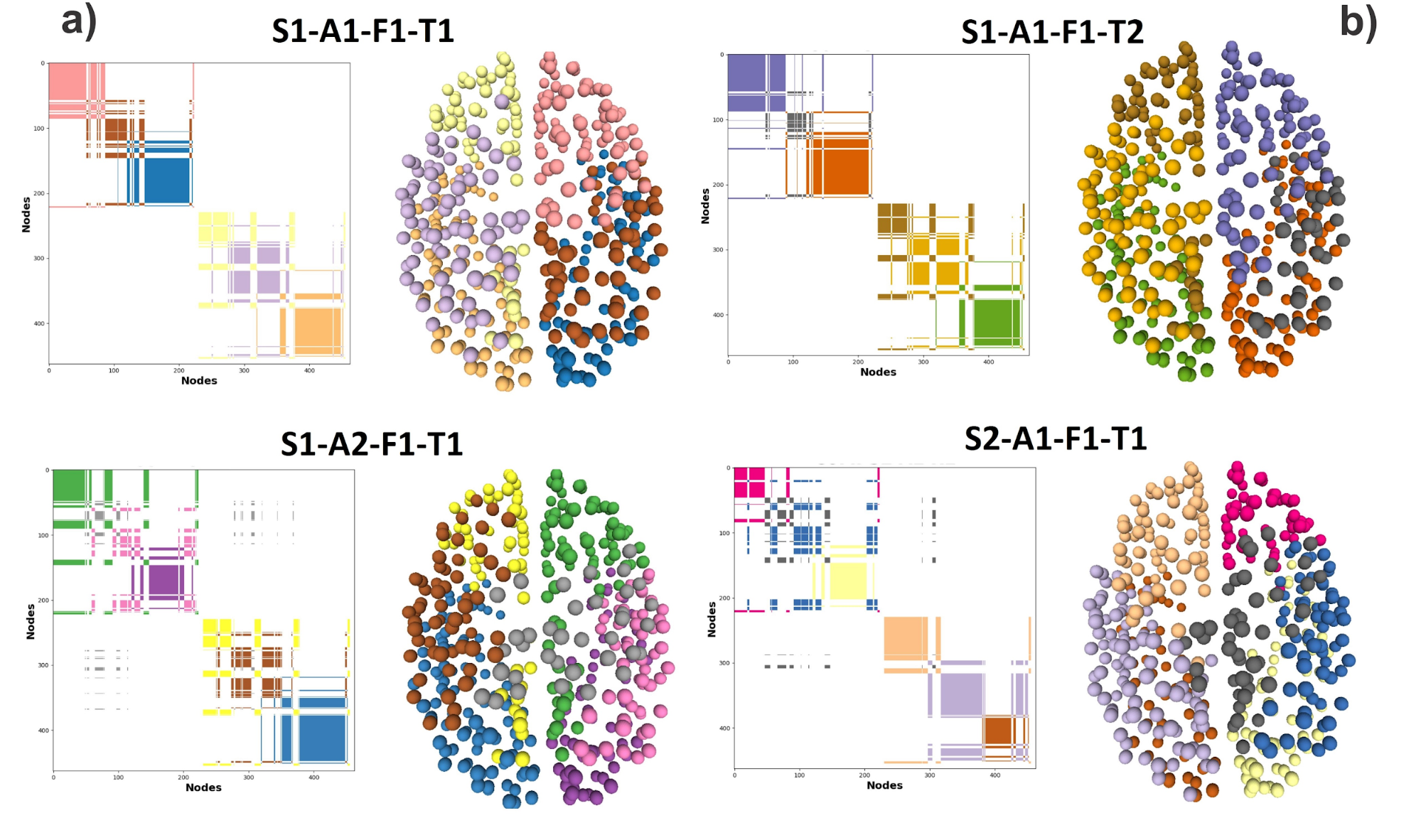
In complex networks, the graph communities are a partition of nodes divided by their connectivity attributes. The community structure is formed by those sets of nodes with dense intra-set connectivity and scattered inter-set connections. Our case of study is the brain's structural connectomes derived from DW-MRI tractography [4]. In the connectome, the communities represent local neighborhoods in the topological connectivity of the brain network. To study the Community structure, we build the Community Matrix, whose format, described in Figure 1, is similar to the adjacency matrix.Detecting the brain regions that interact with each other has applications for brain development, functional organization analysis, and disease detection [5]. Although the communities have been widely studied [5], little has been done to study its estimation reproducibility and per subject's variability.
Here, we propose a novel methodology to analyze node-wise variability induced by changes in connectome-pipelines. We study the graph's noise introduced by: the acquisition, the image processing pipeline, the voxel-wise diffusivity modeling, the tractography parameters, the volume registration, and graph construction parameters.
Methods
Database: We use the DW-MRI datasets from [1], the image pre-processing, and the connectome pipeline are described in [3]. The structural graph weights are derived from the COMMIT framework [6], which provides a quantitative assessment of the proportion of white matter tissue connecting cortical regions.To properly analyze the connectivity estimation variability, we used the following database of 180 connectomes: ten subjects (S_i), three acquisitions (A_j) per subject, three sets of Fiber Orientation Distributions (FOD) images (F_k), and two tractograms per FOD image (T_m). When measuring distances between two connectomes, the comparison will fall into one of the following variabilities classes: Tracto-var, connectomes that differ by tractography; FOD-var, that vary by reconstruction of FOD image; Acqui-var, by different Subject Acquisition session; Subject-var, connectomes from multiple subjects.
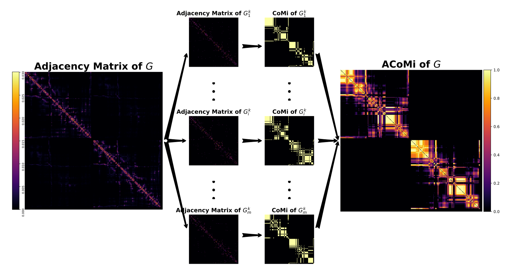
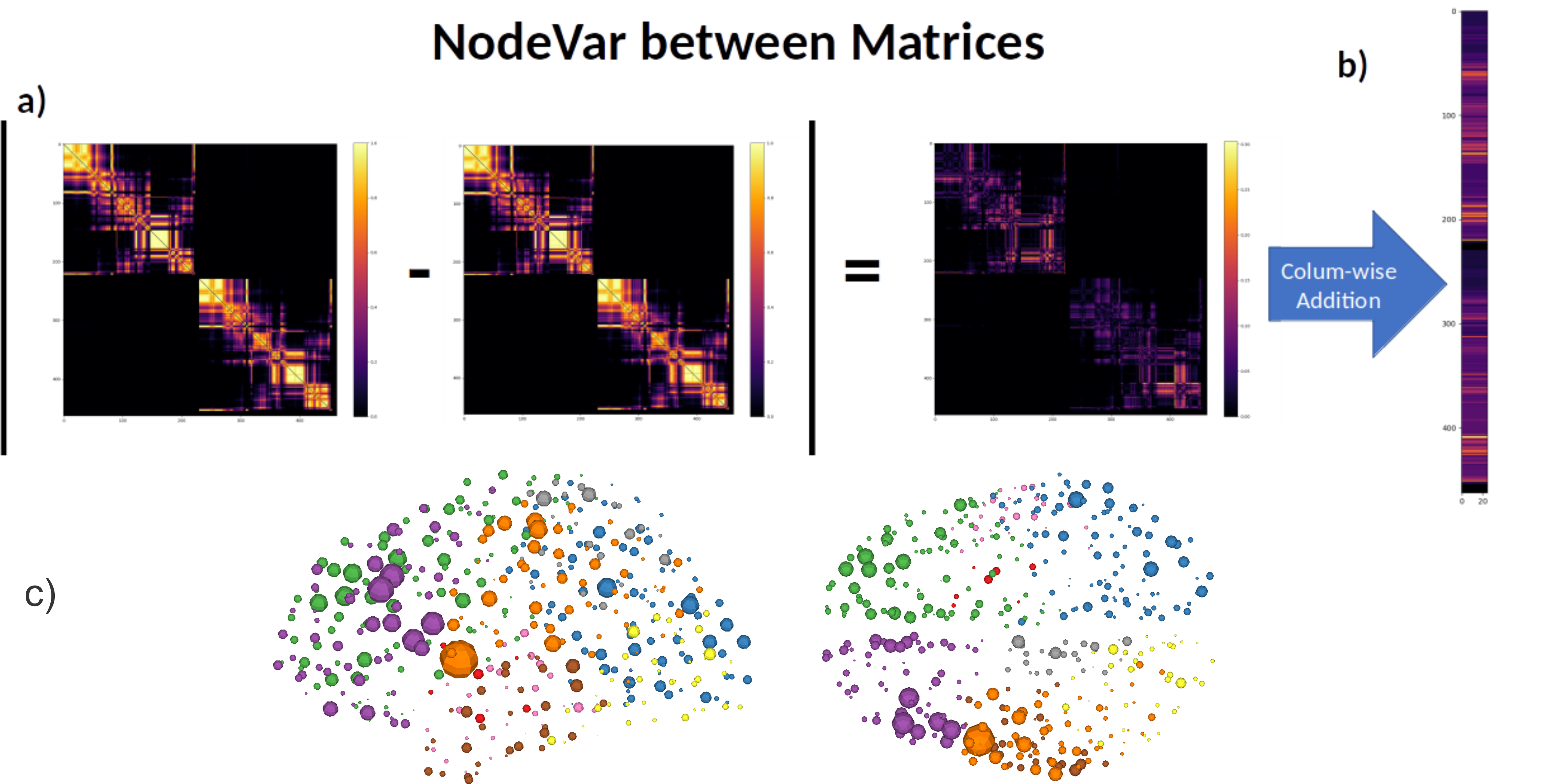
Measures. To measure nodes' persistence to a community, we used the Averaged-Community-Matrix (ACoMi)[3]feature used Monte-Carlo simulations to estimate the node's probability of belonging to different communities. It uses the topological connectivity information of the whole network to retrieve the robust characteristics of the community organization. NodeVar, which calculates the differences in the weighted-degree-distribution between two matrices' features. The higher the NodeVar of a node, the more different the nodes' connectivity profile in the selected matrix feature (Adjacency Matrix or ACoMi). We use the NoderVar index to highlight the connectivity changes due to modifications in the connectomes' pipeline.
Results-and-Discussion
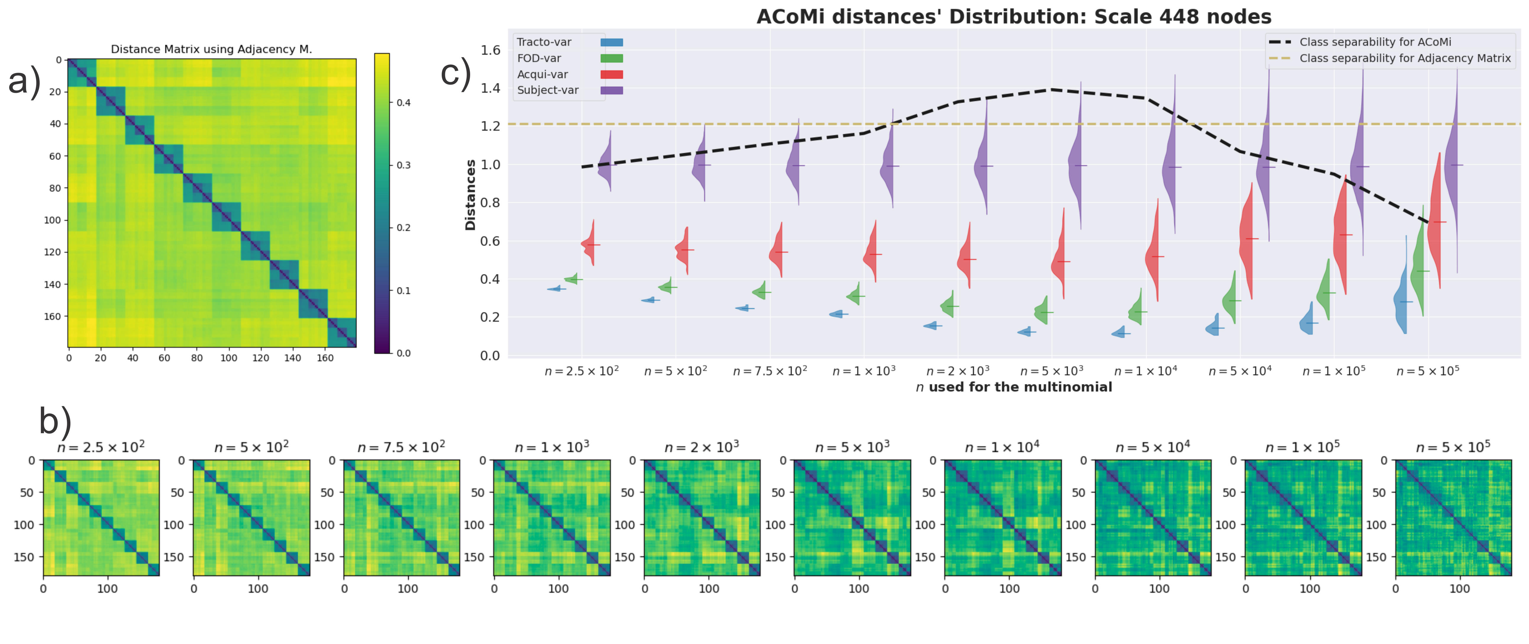
The connectome's community-estimation is sensitive to construction parameters. Figure 1 shows the changes in Subject_1's community structure when one step in the pipeline is repeated. To gather a more robust profile in the community structure, we use the ACoMi, explained in Figure 2. Then, in Figure 3, we studied the ACoMi's efficiency in the following cases: to 1) separate subjects, 2) minimize distances between connectomes computed from the pipeline's repetitions. Figure 3 c) shows that the ACoMi outperforms the adjacency matrix in the cases of 1) and 2) when measuring distances between connectomes.As explained in Figure 3, the analysis consists of tuning a parameter $n$ from a multinomial distribution. The $n$ is responsible for the variance used to create the Monte-Carlo simulations used in the experiments. Then the ACoMis are built using just one optimal $n$. Future work will include the usage of multiple $n$ to increase the quality and quantity of extracted features when calculating the ACoMi.
Then, Figure 4 shows how to build the NodeVar using two ACoMis. The NodeVar is useful to determine the more susceptible-to-error brain nodes. Not all nodes are affected simultaneously; some brain areas are more susceptible to accumulate errors when changing steps within the pipeline. Hence, we could make further studies paying extra attention to those regions with higher differences. Note that Figure 4 is made just for one comparison of two connectomes.
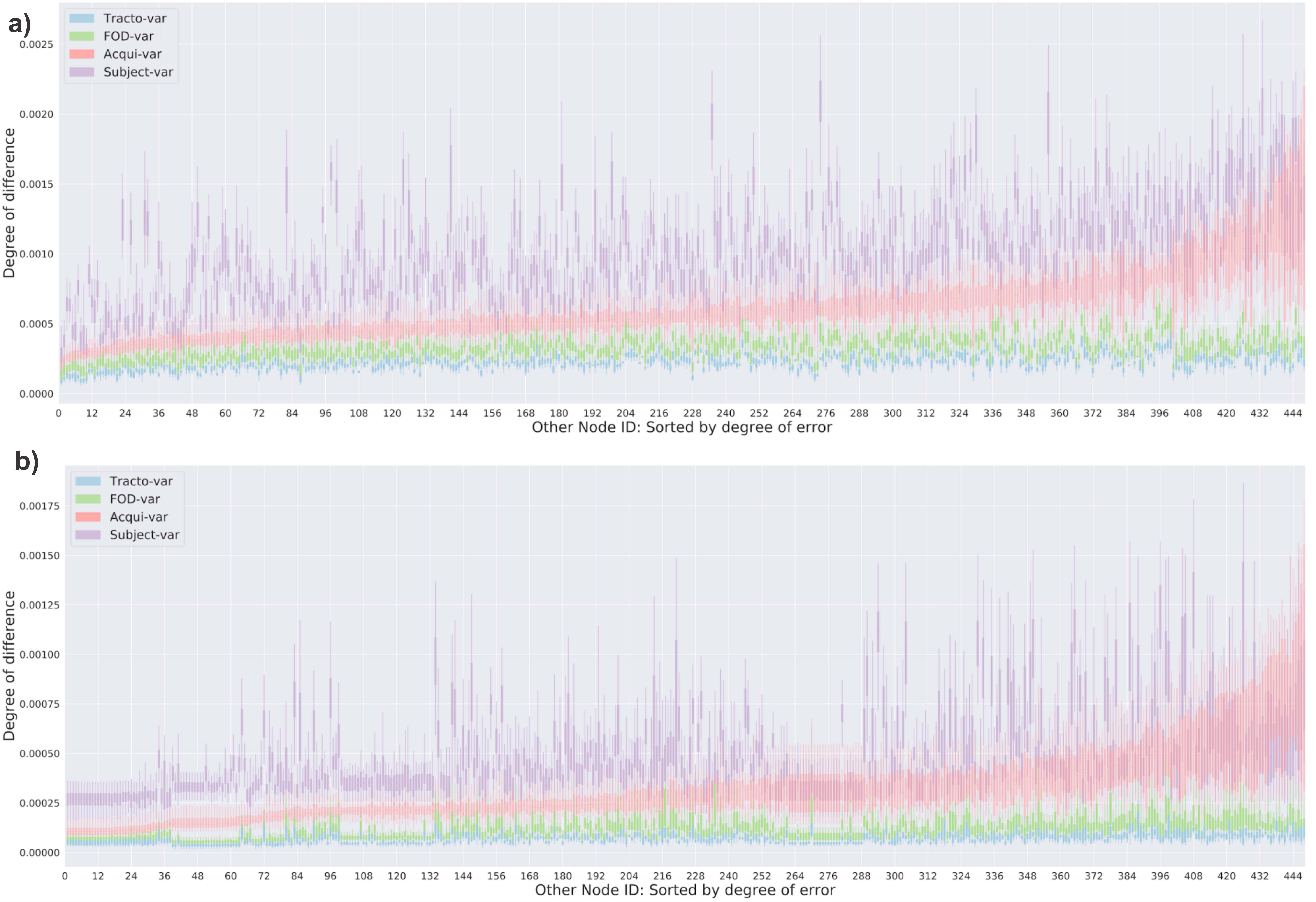
In Figure 5, we use NodeVar of the whole possible pairwise comparisons of the 180 connectomes, which gives us extra statistical power to identify the nodes with the most changes. Furthermore, we can classify the NodeVar values into the variability classes of Tracto-var, FOD-var, Acqui-var, and Subject-var. The result shows that, using the ACoMi, all nodes are relatively stable when doing tractography repetitions or recomputing the FOD maps. However, there are some considerable changes in the connectivity structure of the connectomes that differ by Acquisition. Finally, the nodes with higher NodeVar values in the Subject-var class are a notable change in the structural connectivity between different subjects. In future work, patient datasets will be used to study the brain's structural changes because of the pathology.
Conclusions
As a result of our analysis, we observe which structure of the graph communities is robust to the pipeline changes. Moreover, it provides information about those brain regions more susceptible to accumulated error, and it identifies the robust regions in the reconstruction. Despite the cumulative errors in the graph reconstruction (recomputing tractography, re-estimating FOD maps, changing acquisition sessions, volume registrations), this study provides information that could improve the detection of error in the brain-graph pipeline.Acknowledgements
No acknowledgement found.References
[1] Chamberland, M., Bernier, M., Girard, G., Fortin, D., Descoteaux, M., & Whittingstall, K. (2019). Penthera 1.5T. https://doi.org/10.5281/ZENODO.2602022
[2] Martínez, J. H., & Chavez, M. (2019). Comparing complex networks: in defense of the simple. New Journal of Physics, 21(1), 013033.
[3] Villarreal-Haro J.L. Girard G., Thiran J.P., Ramirez-Manzanares A. A novel robust network community identification method for structural connectome analysis. OHBM, 2020
[4]Hagmann, P., Kurant, M., Gigandet, X., Thiran, P., Wedeen, V. J., Meuli, R., & Thiran, J.-P. (2007). Mapping human whole-brain structural networks with diffusion MRI. PloS One, 2(7), e597. https://doi.org/10.1371/journal.pone.0000597
[5]Bullmore, E., & Sporns, O. (2009). Complex brain networks: graph theoretical analysis of structural and functional systems. Nature Reviews Neuroscience, 10(3), 186–198. https://doi.org/10.1038/nrn2575
[6] Daducci, A., Dal Palù, A., Lemkaddem, A., & Thiran, J. P. (2014). COMMIT: convex optimization modeling for microstructure informed tractography. IEEE transactions on medical imaging, 34(1), 246-257.
Figures