1640
An investigation into the optimal undersampling parameters for 3D TOF MRA at 7T using compressed sensing reconstruction1Wellcome Centre for Integrative Neuroimaging, FMRIB Division, Nuffield Department of Clinical Neurosciences, University of Oxford, Oxford, United Kingdom, 2Oxford Centre for Clinical Magnetic Resonance Research, Department of Cardiovascular Medicine, University of Oxford, Oxford, United Kingdom
Synopsis
3D TOF-MRA at 7T can be greatly accelerated using compressed sensing reconstruction of undersampled acquisitions, but the achieved reconstruction quality depends on the undersampling pattern. In this work, optimal parameters for variable-density Poisson disk undersampling were established. For all acceleration factors, optimal reconstructions were achieved by using small fully-sampled calibration areas of 12x12 lines and a polynomial order of around 2. The optimal undersampling parameters were the same for all acceleration factors, but the importance of using optimized undersampling parameters was found to increase for higher acceleration factors.
Introduction
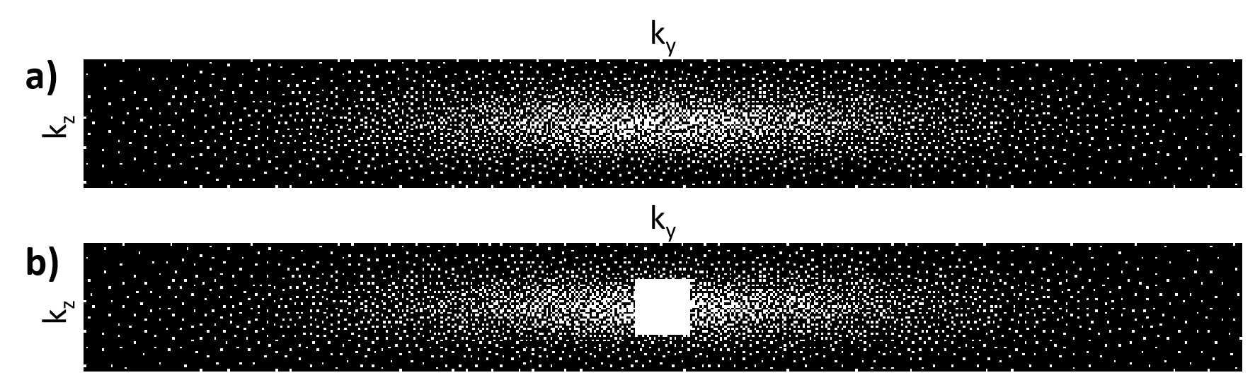
Time-of-flight (TOF) magnetic resonance angiography (MRA) is a common clinical technique for visualisation of the intracranial vasculature. High spatial resolution MRA can visualize small and highly tortuous vessels such as the lenticulostriate arteries1, which are implicated in up to a third of symptomatic strokes2. In order to achieve practical scan times, compressed sensing (CS) reconstruction can be used to iteratively reconstruct highly undersampled data3. However, the accuracy of CS reconstructions depends on the undersampling patterns being used.Cartesian undersampling trajectories in 3D are commonly designed using two-dimensional undersampling masks covering the two phase-encode directions, with each sampled point representing a continuously sampled line in the frequency-encode direction (kx). Undersampling masks are often generated using pseudo-random variable-density Poisson disks4 with a fully-sampled auto-calibration region in the centre of k-space5-9. Variable-density Poisson-disk undersampling distributions are characterized by three parameters: the undersampling factor (equivalent to the acceleration factor, R), the polynomial order of the sampling density variation (pp), and the size of the fully-sampled auto-calibration region: see Figure 1. Although the reconstruction quality depends on those undersampling parameters, no conclusive information is available about their optimal values for 3D TOF-MRA at 7T.
In this work, optimal 3D TOF-MRA undersampling parameters were established for various acceleration factors at 7T through reconstruction of retrospectively undersampled data. The results were subsequently validated using additional prospectively undersampled acquisitions that adopted the optimized parameters.
Methods
Data were acquired using a 3D gradient-echo non-contrast-enhanced TOF-MRA sequence on a Siemens (Erlangen, Germany) Magnetom 7T scanner using a 1Tx, 32-channel Rx head-coil (Nova Medical, Wilmington, Massachusetts). Two healthy subjects were scanned to generate the data used for initial optimization, comprising 4 slabs with a total field-of-view of 220x174x60mm and resolution of 0.34mm isotropic. Further sequence parameters were: TR/TE 14ms/5.61ms, flip angle 20o, bandwidth 118 Hz/pixel, and a total acquisition time of 27 minutes for a fully-sampled acquisition. For validation of the retrospective optimization results, further prospectively undersampled and fully-sampled datasets were acquired from three additional healthy subjects.Coil sensitivities were estimated using ESPIRiT10, and compressed sensing was implemented using the BART-toolbox12,13 (v0.4.02) using FISTA11 with l1 wavelet-regularization. Reconstructions were performed using λ=0.07 in the wavelet domain with 20 iterations, which yielded consistently good reconstruction results for various undersampled datasets in an initial reconstruction parameter optimization.
The quality of the different undersampled reconstructions, relative to the fully sampled reconstructions, was quantitatively assessed using the intracranial vessel-masked structural similarity index (SSIM), which has been found previously to correlate well with visual evaluation by radiologists14.
Results
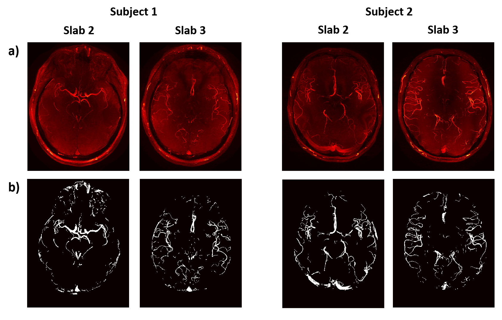
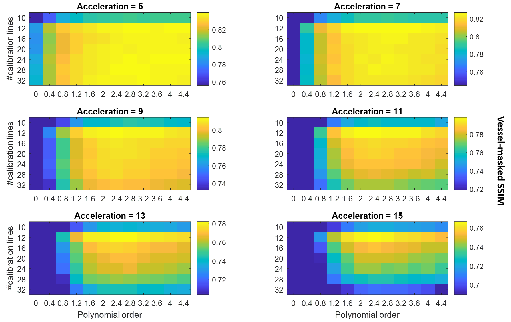
Figure 2 shows fully-sampled reconstructions and the corresponding vessel masks for the four slabs that are used for all retrospectively undersampled reconstructions.The results of undersampling parameter optimization are shown in Figure 3, which indicates an optimal set of undersampling parameters at calib = 12 (i.e. 12x12 calibration lines) with a polynomial order of approximately 2. This result is particularly evident for higher acceleration factors.
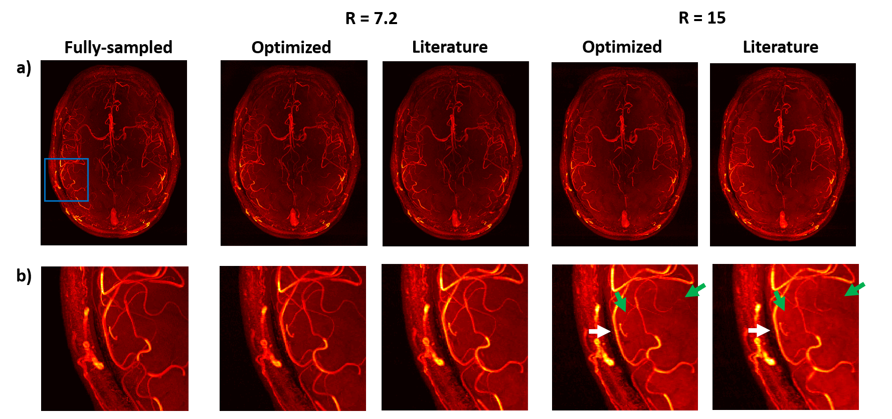
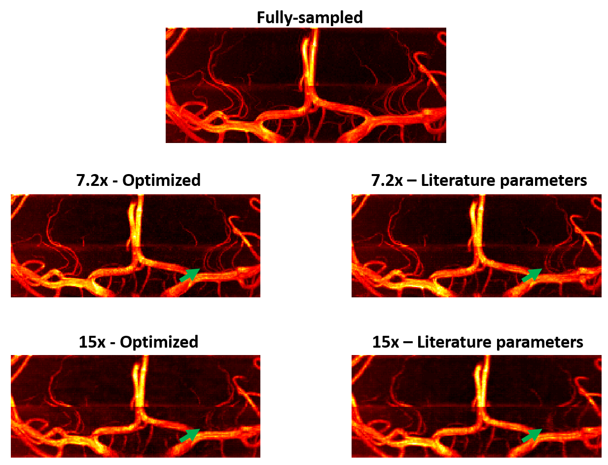
Figures 4 and 5 show reconstructions from fully-sampled data and prospectively undersampled data, using both (i) those ‘optimal’ undersampling parameters and (ii) calibration region sizes based on values found in the literature5 (representative data is shown from a single subject). Results are shown for an acceleration factor of 7.2 (which was previously found to be “a reasonable trade-off between scan time and image quality”5), and a higher acceleration factor of 15.
Discussion
Although differences in the reconstruction accuracy for different sets of parameters are visible for all acceleration factors in Figure 3, the relative importance of using the optimal parameters increases with higher acceleration factors. For all acceleration factors the combination of 12x12 calibration lines with a polynomial order of about 2 consistently yielded the best reconstruction accuracy. This optimal calibration region size is considerably smaller than values found in the literature, and makes it possible to spend more scan time acquiring high spatial frequency-data.Figures 4 and 5 show a clear reduction in the number of visible vessels both for optimized and literature-based acquisition parameters at higher acceleration. However, the vessel visibility and sharpness is consistently superior when using optimized undersampling parameters. This improvement can be achieved without increasing scan time or reconstruction time, and without additional technical requirements.
The data used in this work were acquired using a relatively simple protocol. Alternative protocols may result in changes to the acquired contrasts. However, the optimal undersampling parameters were found to be consistent for volumes with high differences in vascular characteristics and visibility (Figure 2). When acquiring data at different resolutions, the optimal polynomial order could change accordingly but the required calibration region size for accurate coil sensitivity estimation is expected to remain consistent. Although 32-channel receive coils are most commonly used in 7T MRI, it remains unclear how the results presented here would translate to different coil configurations.
Conclusion
Optimal undersampling parameters for 3D MRA at 7T using compressed sensing reconstruction were established. For all acceleration factors, optimal reconstructions were achieved by using a fully-sampled calibration area of 12x12 lines and a polynomial order of around 2. Although the optimal undersampling parameters were the same for all acceleration factors, the importance of using optimized undersampling parameters was found to increase for higher acceleration factors.Acknowledgements
MdB receives financial support from Siemens Healthineers and the Dunhill Medical Trust.References
[1] J. Hendrikse, J. J. Zwanenburg, F. Visser, T. Takahara, and P. Luijten, “Noninvasive depiction of the lenticulostriate arteries with time-of-flight MR angiography at 7.0 T,” Cerebrovasc. Dis., vol. 26, no. 6, pp. 624–629, 2008.
[2] S. M. Greenberg, “Small Vessels, Big Problems,” N. Engl. J. Med., vol. 354, no. 14, pp. 1451–1453, 2006.
[3] M. Lustig, D. Donoho, and J. M. Pauly, “Sparse MRI: The application of compressed sensing for rapid MR imaging,” Magn. Reson. Med., vol. 58, no. 6, pp. 1182–1195, 2007.
[4] B. Deka and S. Datta, “A Practical Under-Sampling Pattern for Compressed Sensing MRI,” Lect. Notes Electr. Eng., vol. 347, pp. 115–125, 2015.
[5] C. R. Meixner et al., “High resolution time-of-flight MR-angiography at 7 T exploiting VERSE saturation, compressed sensing and segmentation,” Magn. Reson. Imaging, vol. 63, no. August, pp. 193–204, 2019.
[6] T. Yamamoto et al., “Magnetic resonance angiography with compressed sensing: An evaluation of moyamoya disease,” PLoS One, vol. 13, no. 1, pp. 1–11, 2018.
[7] S. Rapacchi et al., “High spatial and temporal resolution dynamic contrast-enhanced magnetic resonance angiography using compressed sensing with magnitude image subtraction,” Magn. Reson. Med., vol. 71, no. 5, pp. 1771–1783, 2014.
[8] K. G. Hollingsworth, “Reducing acquisition time in clinical MRI by data undersampling and Compressed Sensing reconstruction,” Phys. Med. Biol., vol. 60, no. 21, pp. R297–R322, 2015.
[9] M. H. Moghari, M. Uecker, S. Roujol, M. Sabbagh, T. Geva, and A. J. Powell, “Accelerated whole-heart MR angiography using a variable-density poisson-disc undersampling pattern and compressed sensing reconstruction,” Magn. Reson. Med., vol. 79, no. 2, pp. 761–769, 2018.
[10] M. Uecker et al., “ESPIRiT - An eigenvalue approach to autocalibrating parallel MRI: Where SENSE meets GRAPPA,” Magn. Reson. Med., vol. 71, no. 3, pp. 990–1001, 2014.
[11] A. Beck and M. Teboulle, “A Fast Iterative Shrinkage-Thresholding Algorithm,” Soc. Ind. Appl. Math. J. Imaging Sci., vol. 2, no. 1, pp. 183–202, 2009.
[12] BART Toolbox for Computational Magnetic Resonance Imaging, DOI: 10.5281/zenodo.592960.
[13] J. I. Tamir, F. Ong, J. Y. Cheng, M. Uecker, and M. Lustig, “Generalized Magnetic Resonance Image Reconstruction using The Berkeley Advanced Reconstruction Toolbox,” Proc. ISMRM 2016 Data Sampl. Image Reconstr. Work., vol. 2486, 2016.
[14] T. Akasaka et al., “Optimization of regularization parameters in compressed sensing of magnetic resonance angiography: Can statistical image metrics mimic radiologists’ perception?,” PLoS One, vol. 11, no. 1, pp. 1–14, 2016.
Figures