1561

Sequence Optimisation for Multi-Component Analysis in Magnetic Resonance Fingerprinting

David Heesterbeek^1,2, Frans Vos^1,3, Martin van Gijzen², and Martijn Nagtegaal¹
¹Department of Imaging Physics, Delft University of Technology, Delft, Netherlands, ²Department of Numerical Analysis, Delft University of Technology, Delft, Netherlands, ³Department of Radiology and Nuclear Medicine, Erasmus MC, Rotterdam, Netherlands

Synopsis

Quantitative MRI and especially MR Fingerprinting make use of complicated acquisition schemes and signal models to measure tissues parameters. The sequence choice is crucial for the noise robustness for parameter estimations of different tissues. Multi-component (MC) signal models for MRF are of importance to estimate partial volume effects or myelin water fractions for example. We propose to use the Cramér-Rao bound to assess and optimise the multi-component parameter estimations for MRF. The optimised flip angle and TR patterns for MC-MRF were highly structured which was also observed for the optimisation based on the single-component model, but structural differences were noticed.

Introduction

Quantitative Magnetic Resonance Imaging has the potential to improve the reproducibility of MRI measurements by taking confounding physical processes into account that underlie the MR signal. In MR Fingerprinting (MRF)[1] a transient state signal is acquired, such that multiple relevant tissue parameters as well as system properties can be estimated simultaneously.

MRF typically consists of a flexible framework in which pseudo randomised acquisition patterns with varying length, flip angles(FA) and repetition times(TR) are applied. These encoding parameters can be optimised using different criteria e.g. by maximising the orthogonality of the dictionary signals[2] or reducing the Cramér-Rao bound(CRB) to improve the signal-to-noise ratio (SNR)[3,4]. In effect this can lead to enhanced measurement precision and/or a reduction in scan time.

These single-component optimisations do not necessarily improve estimations when multiple tissues are present in one voxel. A multi-component model is required, when estimating e.g. the myelin water fraction in white matter, a relevant parameter in many diseases such as multiple sclerosis, schizophrenia and concussions[5], or on boundaries between white matter, grey matter or CSF. In multi-component analysis the mixing of signals from different tissues in one voxel is taken into account. Current efforts in multi-component MRF (MC-MRF) focus on finding an optimal solution to a linear inverse problem[6,7] using standard MRF sequences. The choice of FA and TR patterns can, however, influence the precision of the multi-component analysis. In this work we introduce a framework for quantifying and optimising the precision of a chosen acquisition sequence based on the CRB specifically for MC-MRF.

Methods

The CRB is an estimation-theoretical limit to the precision with which a parameter can be estimated using an unbiased estimator. As such the CRB makes it possible to quantitatively compare different MRF sequences[3], and is determined by the inverse of the Fisher information matrix $$$\boldsymbol{F}$$$.

To model the spin dynamics the Extended Phase Graph (EPG) formalism[8] was used, which typically yields marked computational advantages compared to the isochromat summation approach used in[3].

The MC-MRF signal is modelled as:$$\boldsymbol{s}[n]=\sum_{i}\boldsymbol{m}_{i}(T_{1}^{x_{i}},T_{2}^{x_{i}},M_{0}^{x_{i}})[n]+\boldsymbol{w}[n],$$where $$$\boldsymbol{s}[n]$$$ is the measured magnetisation at the $$$n$$$th read-out time, $$$\boldsymbol{m}_{i}[n]$$$ is the theoretical transverse magnetisation in the absence of noise for tissue $$$x_{i}$$$ at the $$$n$$$th read-out time and $$$\boldsymbol{w}[n]$$$ is independent identically distributed Gaussian noise. For the single-component model $$$i$$$ concerns a single index.

Sequence optimisation for the single-component model is performed for a limited set of parameters, i.e. $$$T_{1},~T_{2}$$$ and $$$M_{0}$$$[3]. However, for the multi-component optimisation, the number of parameters for which we optimise scales linearly with the number of tissues considered. When two tissues are considered these parameters are $$$T_{1}^{a},~T_{2}^{a},~M_{0}^{a},~T_{1}^{b},~T_{2}^{b}$$$ and $$$M_{0}^{b}$$$ where the superscript is meant to distinguish different tissues.

Using the multi-component model the weighted sum of the CRBs can be minimised by optimising the acquisition parameters FA ($$$\alpha$$$) and TR for a sequence (length $$$N$$$), using empirically defined constraints:$$\min_{\{\alpha_n,TR_n\}_{n=1}^{N}}\quad\sum_{i=1}^{6}w_{i}\cdot~F(T_{1}^{a},T_{2}^{a},M_{0}^{a},T_{1}^{b},T_{2}^{b}, M_{0}^{b})^{-1}_{i, i}$$$$\textrm{s.t.}\quad~10^{\circ}\leq\alpha_{n}\leq 60^{\circ}~\forall~n\in\{2,3,..,N\}$$$$11~\text{ms}\leq TR_{n}\leq~15\text{ ms}~\forall~n\in\{1,2,..,N\}$$$$|\alpha_{n+1}-\alpha_{n}|\leq 1^{\circ}~\forall~n\in\{1,2,...,N-1\}$$where $$$w$$$ is a weighting factor. The first two constraints enable both that results are unique as well as clinically feasible while the last constraint is set in place to keep the evolution of the magnetisation smooth which is beneficial in virtually all decoding schemes.This non-linear constrained optimisation problem is solved by using a Sequential Least-Squares Quadratic Programming algorithm.

Results

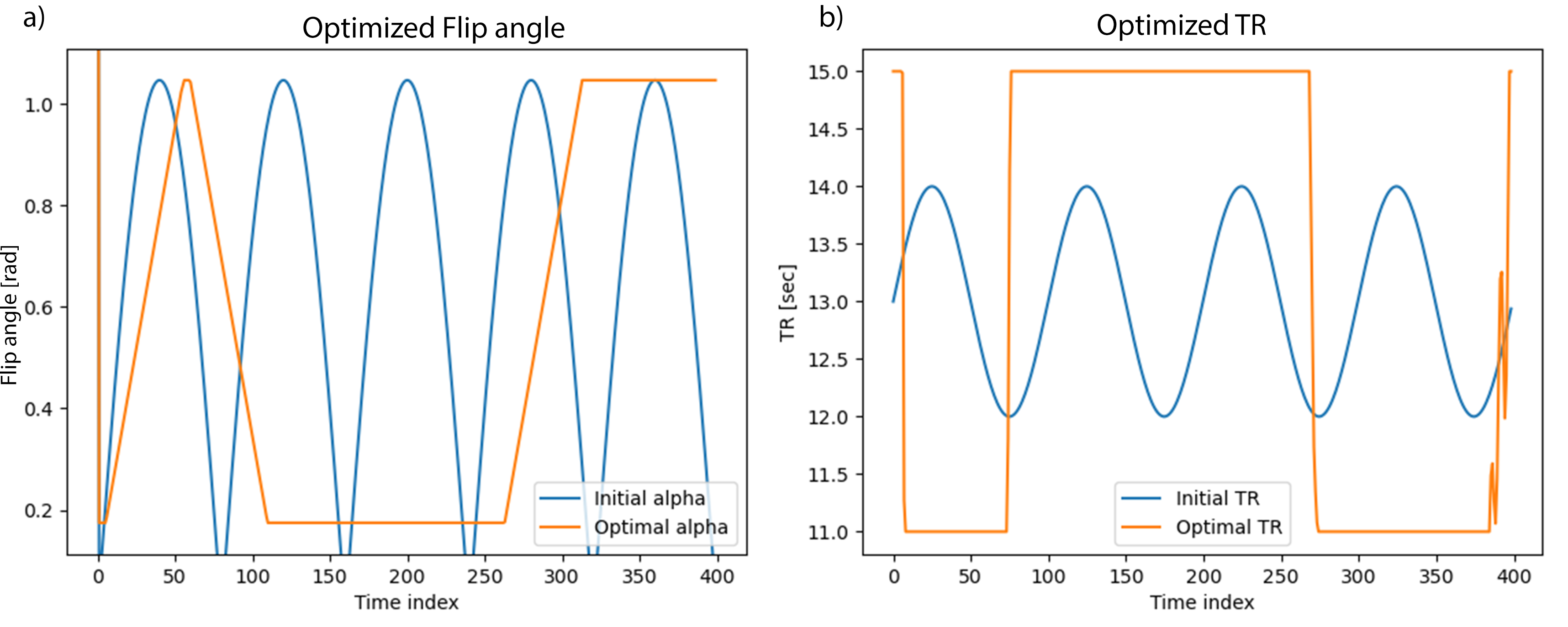
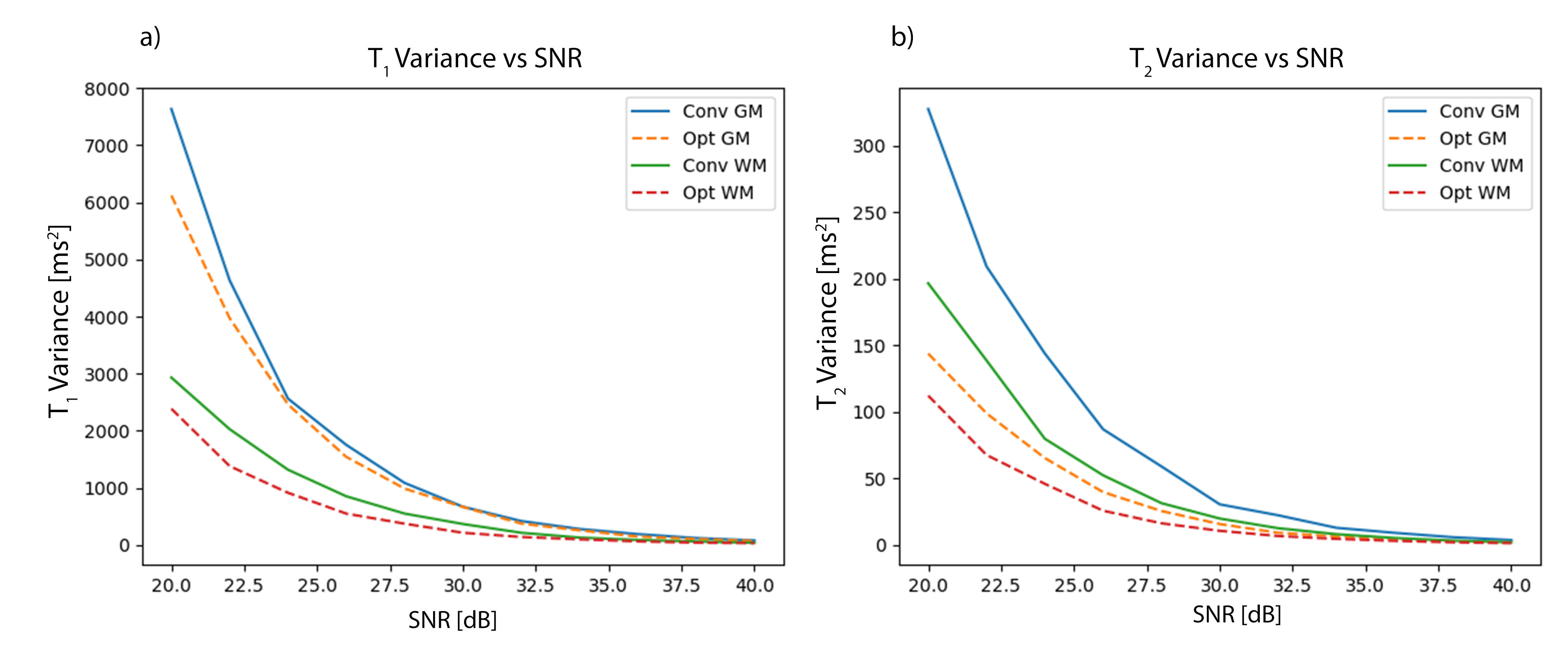
Numerical optimisation of the CRB using a single-component model and EPG for an MRF-IR-FISP[9] sequence is shown in Fig.1. These results are extremely similar to the results in[3] for the same problem.

The variance in estimated $$$T_1$$$ and $$$T_2$$$ of grey and white matter, using the conventional (see initialisation Fig.1) and optimised sequence, for different SNRs is shown in Fig.2.

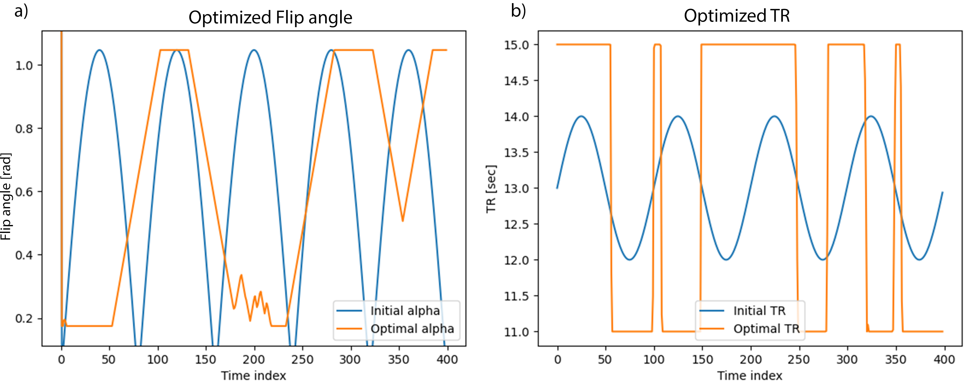
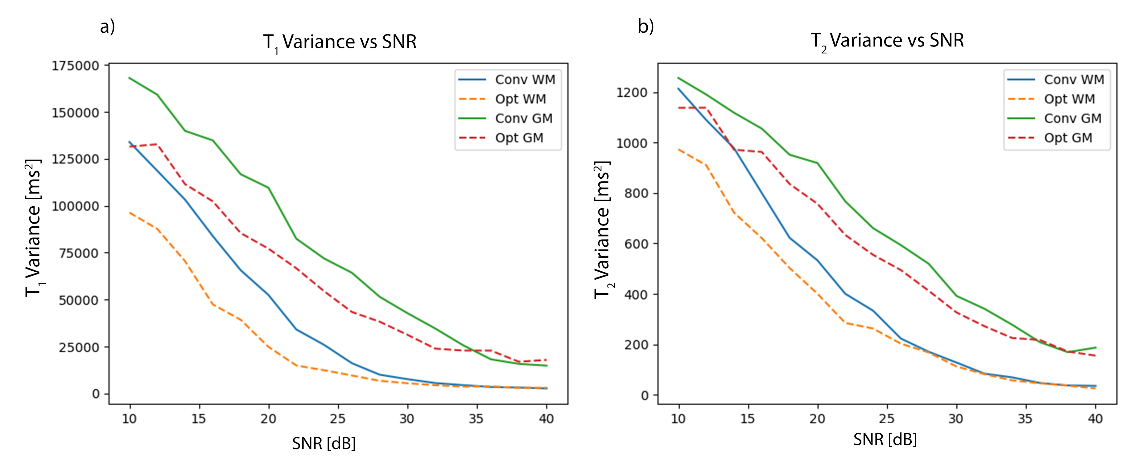
Similarly, the optimised parameters and variance in $$$T_1$$$ and $$$T_2$$$ for MC-MRF are shown in Fig.3 and Fig.4.

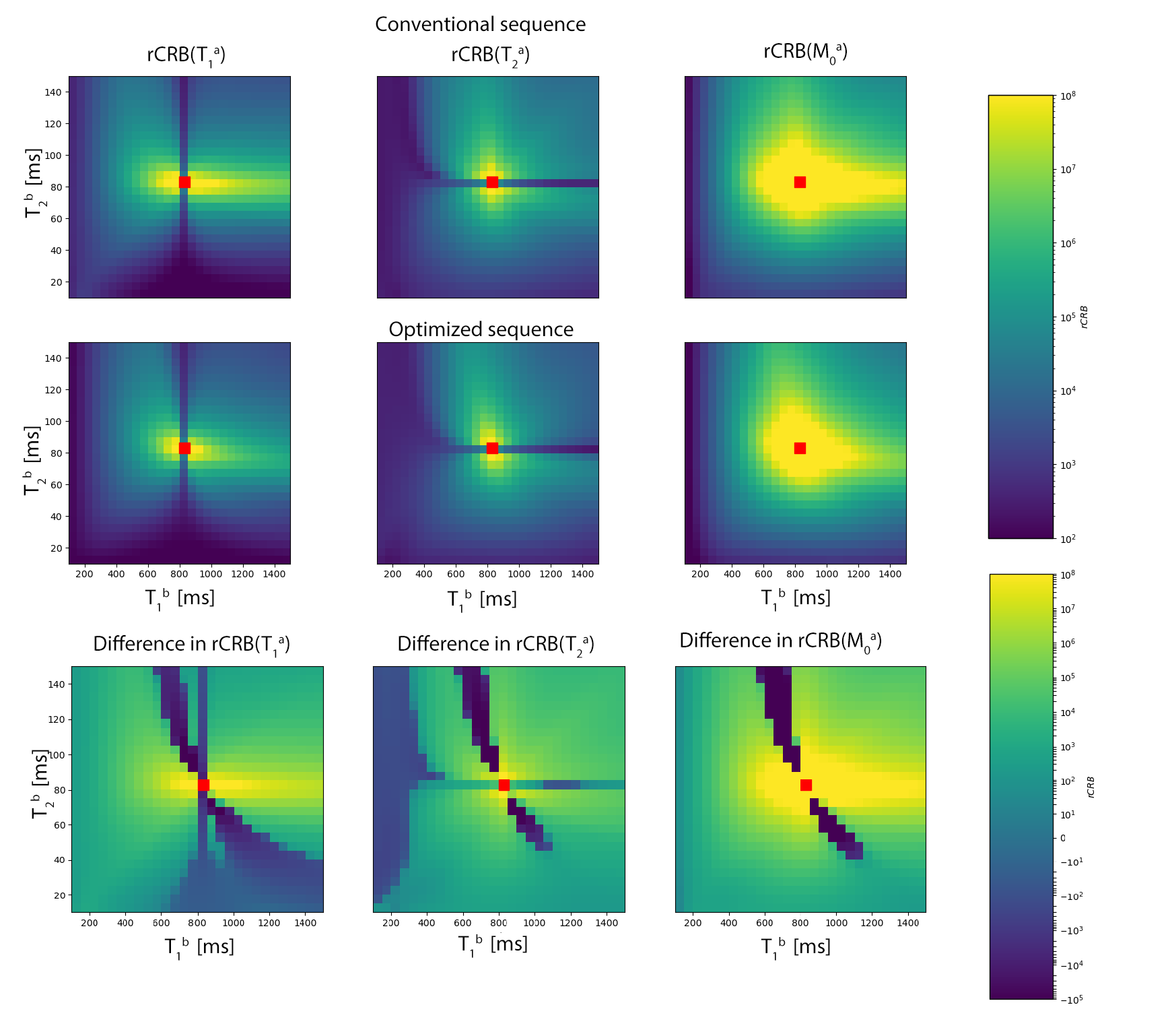
CRB evaluation for MC-MRF for different $$$T_{1}$$$-$$$T_{2}$$$ combinations for the conventional and optimised sequence are shown in Fig.5. The difference(row 3) shows that the optimised sequence generally gives a lower rCRB, as we expected. The figure shows that the rCRB of a parameter increases if this parameter for tissue b approaches the value of tissue a. The horizontal and vertical lines however, show that if the parameters are equal the rCRB decreases. Intuitively this marks the transition from being hard to distinguish (prone to errors) to being exactly the same (comparable to estimating one tissue using a single-component model).

Discussion and Conclusion

We introduced an optimisation method based on the theoretical CRB for MC-MRF. Its usefulness was shown in the application to different MRF-FISP sequences using the multi-component model. Further comparisons can be made with other regular sequences used for multi-component estimations such as multi-echo spin echo and mcDESPOT.
Monte Carlo simulations showed that improvements could be obtained in multi-component estimations by sequence optimisation. In future work we will perform in vitro and in vivo scans to assess the achieved improvement in precision in practice.
The results were optimised for white and grey matter relaxation times, in further studies we plan to optimise for different tissues such as myelin water and CSF.

In conclusion, the Cramér-Rao Bound shows to serve as a tool in multi-component models to quantitatively assess and optimise different sequences. This method provides new insights into the possibilities and restrictions of multi-component estimations.

Acknowledgements

M.A. Nagtegaal his research is funded by the Medical Delta consortium, a collaboration between the Delft University of Technology, Leiden University, Erasmus University Rotterdam, Leiden University Medical Center and Erasmus Medical Centre.

References

[1] Dan Ma, Vikas Gulani, Nicole Seiberlich, Kecheng Liu, Jeffrey L.Sunshine, Jeffrey L. Duerk, and Mark A. Griswold. Magnetic Resonance Fingerprinting. Nature, 495(7440):187–192, March 2013.

[2] Ouri Cohen and Matthew S. Rosen. Algorithm comparison for schedule optimization in MR fingerprinting. Magnetic Resonance Imaging, 41:15–21, September 2017.

[3] B. Zhao, J. P. Haldar, C. Liao, D. Ma, Y. Jiang, M. A. Griswold, K. Setsompop, and L. L. Wald. Optimal Experiment Design for Magnetic Resonance Fingerprinting: Cramér-Rao Bound Meets Spin Dynamics. IEEE Transactions on Medical Imaging, 38(3):844–861, March 2019.

[4] Jakob Assländer, Riccardo Lattanzi, Daniel K. Sodickson, and Martijn A. Cloos. Optimized quantification of spin relaxation times in the hybrid state. Magnetic Resonance in Medicine, June 2019.

[5] Alex L. MacKay and Cornelia Laule. Magnetic Resonance of Myelin Water: An in vivo Marker for Myelin. Brain Plasticity, 2(1):71–91, 2016.

[6] Debra F. McGivney, Rasim Boyacıoglu, Yun Jiang, Megan E. Poorman, Nicole Seiberlich, Vikas Gulani, Kathryn E. Keenan, Mark A. Griswold, and Dan Ma. Magnetic resonance fingerprinting review part 2: Technique and directions. Journal of Magnetic Resonance Imaging, 51(4):993–1007, July 2019.

[7] Martijn Nagtegaal, Peter Koken, Thomas Amthor, and Mariya Doneva. Fast multi-component analysis using a joint sparsity constraint for MR fingerprinting. Magnetic Resonance in Medicine, 83(2):521–534, July 2019.

[8] Matthias Weigel. Extended phase graphs: Dephasing, RF pulses, and echoes - pure and simple. Journal of Magnetic Resonance Imaging, 41(2):266–295, February 2015.

[9] Yun Jiang, Dan Ma, Nicole Seiberlich, Vikas Gulani, and Mark A. Griswold. MR fingerprinting using fast imaging with steady state precession (FISP) with spiral readout. Magnetic Resonance in Medicine, 74(6):1621–1631, 2015.

Figures

Figure 1: a) FA and b) TR sequences at initiation and after optimisation for single-component MRF. Optimisation was performed for tissue parameters {$$$T_{1}$$$, $$$T_{2}$$$, $$$M_{0}$$$} = {700ms, 60ms, 0.6}, {850ms, 50ms, 0.6}, {1100ms, 102ms, 0.6} with the constraints mentioned in the Methods section. These optimised patterns are highly similar to the optimised pattern in [3] which was based on an isochromat summation (140 minutes) approach instead of the EPG simulations (40 minutes) as used here.

Figure 2: a) Variance in $$$T_{1}$$$ estimation. b) Variance in $$$T_{2}$$$ estimation. SNR is defined as $$$\text{SNR}=20\text{log}_{10}\frac{M_{0}}{\sigma}$$$. The variance is estimated using a Monte-Carlo approach with 1000 noisy signal realisations per tissue. Grey and white matter are modelled separately using a single-component model.

Figure 3: a) FA and b) TR sequences at initiation and after optimisation for multi-component MRF. Optimisation was performed for tissue parameters {$$$T_{1}^{a}$$$, $$$T_{2}^{a}$$$, $$$M_{0}^{a}$$$} = {700ms, 60ms, 0.3} and {$$$T_{1}^{b}$$$, $$$T_{2}^{b}$$$, $$$M_{0}^{b}$$$} = {1100ms, 102ms, 0.3} with the constraints mentioned in the Methods section. Different initialisation of the optimisation problem returned the same result.

Figure 4: a) Variance in $$$T_{1}$$$ estimation. b) Variance in $$$T_{2}$$$ estimation. The variance is estimated using a Monte-Carlo approach with 1000 realisations. Multi-component estimations were performed using the NNLS algorithm. Grey and white matter are modelled together using a multi-component model.

Figure 5: Relative CRB values were calculated using the multi-component Fisher matrix for a conventional MRF sequence (row 1) and an optimised sequence (row 2). The difference is shown in row 3 by subtracting the second row from the first. The rCRB is defined as $$$\text{rCRB} = \frac{\text{CRB}}{\sigma^2 \theta^2}$$$ where θ represents T₁^a, T₂^a or M₀^a. Tissue parameters for one tissue (superscript a) were fixed at T₁^a= 800 ms, T₂^a= 80 ms, while T₁^band T₂^b for the second tissue (superscript b) vary. In the centre red dot the 2 tissues are exactly the same, resulting in a singularity.

Proc. Intl. Soc. Mag. Reson. Med. 29 (2021)

1561