1559
Uncertainty analysis framework for quantifying error propagation in MR Fingerprinting1Physical Measurement Laboratory, National Institute of Standards & Technology, Boulder, CO, United States, 2Information Technology Laboratory, National Institute of Standards & Technology, Boulder, CO, United States, 3Department of Biomedical Engineering, Case Western Reserve University, Cleveland, OH, United States
Synopsis
This study demonstrated functionality of an error analysis framework applied to understand the impacts of variations in the MR Fingerprinting pipeline. Our preliminary analysis using both simulation and experimental methods showed small differences in the accuracy and precision of the reconstructed property maps with choice of k-space to image space reconstruction method. We demonstrated the need for a better understanding of error propagation within the pipeline, improved quantitative metrics of error, and future work will include a full Monte Carlo analysis using this framework.
Introduction
Magnetic Resonance Fingerprinting1 (MRF) is a tool for quantifying multiple tissue properties simultaneously2,3. The analysis pipeline for an MRF experiment contains many steps, outlined in Figure 1. Each step has flexibility in choice of algorithm and its associated internal parameters. With so many permutations, it is important to understand how variations at each stage affect the stability of resulting tissue property maps.We propose a computational framework used to isolate sources of variability in the MRF pipeline, and to estimate the sensitivity of quantitative property measurements to such variations. The framework allows implementation of pipeline modifications and improvements unique to individual research groups. We present preliminary work demonstrating the uncertainty analysis framework applied to a simulated phantom, and to quantitative analysis of experimental scans of the ISMRM/NIST phantom4.
Methods
Pulse sequence and Dictionary generation:All data was acquired with an SSFP pulse sequence (FISP, FFE, GRASS) using the specified flip angle, repetition time (TR) patterns, and k-space trajectory (Figure 2). The k-space trajectory was rotated 7.5$$$^{\circ}$$$ each TR. A corresponding dictionary was generated using an approximate Bloch solver with ranges T1=[2:2:100, 100:20:2000, 2000:40:3000] and T2=[2:2:130, 130:10:200, 200:20:1000, 1000:40:3000] ms. No B1+ or slice profile corrections were implemented. All data was matched to this dictionary with an exhaustive search algorithm, and the entry with highest correlation to the signal was chosen.
Data acquisition:
A digital phantom containing 12 circles with varying T1 and T2 values was implemented in MATLAB (Mathworks, USA) spanning a 250mm FOV (256x256 matrix, TE=2.2ms). Data was generated using the Bloch solver and pulse sequence described above before undersampling k-space on the spiral in Figure 2, rotated by 7.5$$$^{\circ}$$$ each TR. The generated k-space data was used for analysis.
The ISMRM/NIST phantom was placed in a 16-channel head and neck coil and imaged with a 3T scanner (Siemens Healthcare, Germany) using the described pulse sequence (TE=2.2ms, 256x256 matrix, 250mm FOV). The phantom’s NiCl2 array was imaged with a single 2D slice and used for analysis.
Reconstruction Methods and Analysis:
Both data sets were fed into the pipeline and used to compute T1 and T2 maps. Three different k-space to image space conversion methods were implemented and used as part of the analysis. Method 1 consisted of density compensation followed by an NUFFT using an open-source toolbox5, Method 2 consisted of an NUFFT followed by iterative reconstruction using the same toolbox5, and Method 3 consisted of a multithreaded NUFFT6,7 and a different density compensation method8,9. The property maps resulting from each data set and reconstruction method were compared qualitatively and quantitatively to known values, using an automated ROI selection to compute means and standard deviations within each phantom component.
Results and Discussion
T1 and T2 maps generated from the simulated phantom are displayed in Figure 3; all reconstruction methods are in good visual agreement. Unmasked spiral artifacts are seen outside the circles, substantially infiltrating the objects sitting near the edges of the field of view. All reconstruction methods computed the true T1 and T2 values with less than 10% error (Figures 4A, 4B). The mean percent error respectively for each method was 2.1%, 0.8%, and 5.6% for T1 and 1.7%, 1.0%, and 3.1% for T2. The influence of ROI distance from the center of the phantom can be seen in Figure 4C and 4D and increases with distance from center. This phenomenon could likely be improved by using golden angle rotations on the spiral trajectories.Results from the ISMRM/NIST phantom are displayed in Figure 5. Qualitatively, all reconstruction methods resulted in reasonable T1 and T2 maps (Figure 5A) with little artifact within the phantom. Spiral artifacts were left unmasked outside the phantom to observe influence on the phantom itself. Mean values within each sphere agree with each other to within 9.8 ms average difference in T1 and 13.4 ms average difference in T2 (Figures 5B, 5C). Mean standard deviations across all spheres for Methods 1, 2, and 3, respectively were 20.8, 34.0, and 20.4 ms for T1, and 28.5, 27.9, 27.2 ms for T2. For all spheres, computed mean values deviate from the known NMR values by as much as 20%, which can be expected without B1+ and slice profile corrections10.
This preliminary analysis shows small differences in the accuracy and precision of the reconstructed property maps with choice of k-space to image space reconstruction method. However, the quality of the property maps will be affected by more than one design choice at a time. This demonstrates the need for a better understanding of error propagation within the pipeline, improved quantitative metrics of error, and full Monte Carlo analysis using this framework11.
Conclusions
This study demonstrated functionality of an error analysis framework that can be applied to MRF. The framework will be useful for quantifying how design choices affect the resulting property maps and determining uncertainty bounds. Given the modularity of the pipeline, it could prove useful for testing of novel pipeline modifications and optimization and is highly adaptable to each research group’s needs. Future work aims to fully characterize uncertainty using a Monte Carlo analysis and defining high quality error metrics.Acknowledgements
The authors acknowledge funding from the National Research Council, Siemens Healthineers, Microsoft and NIH grants EB026764-01 and NS109439-01
References
- Ma et. al, “Magnetic Resonance Fingerprinting,” Nature 495(7440) 2013
- Poorman et. al, “Magnetic Resonance Fingerprinting Part 1: Potential uses, current challenges, and recommendations,” JMRI 51(3) 2020
- McGivney et. al, “Magnetic Resonance Fingerprinting Part 2: Technique and directions,” JMRI 51(4) 2020
- Keenan et. al, “NIST/ISMRM MRI System Phantom T1 Measurements on Multiple MRI Systems,” In ISMRM 20th annual meeting Australia 2012
- Fessler, J. , “Michigan Image Reconstruction Toolbox,” https://web.eecs.umich.edu/~fessler/code/
- Barnett et. al, “A Parallel nonuniform fast Fourier transform library based on an “exponential of semicircle” kernel,” SIAM J Sci. Comput. 41(5) 2019
- https://github.com/flatironinstitute/finufft
- Greengard et. al, “The fast sinc transform and image reconstruction from nonuniform samples in k-space,” Comm. App. Math. And Comp. Sci. 1(1) 2006
- Choi and Munson, “Analysis and design of minimax-optimal interpolators,” IEEE Trans. Signal Processing 46 1998
- Ma et. al, “Slice profile and B1 corrections in 2D magnetic resonance fingerprinting,” MRM 78(5) 2017
- Kara et. al, “Parameter map error due to normal noise and aliasing artifacts in Magnetic Resonance Fingerprinting,” MRM 81(5) 2019
Figures
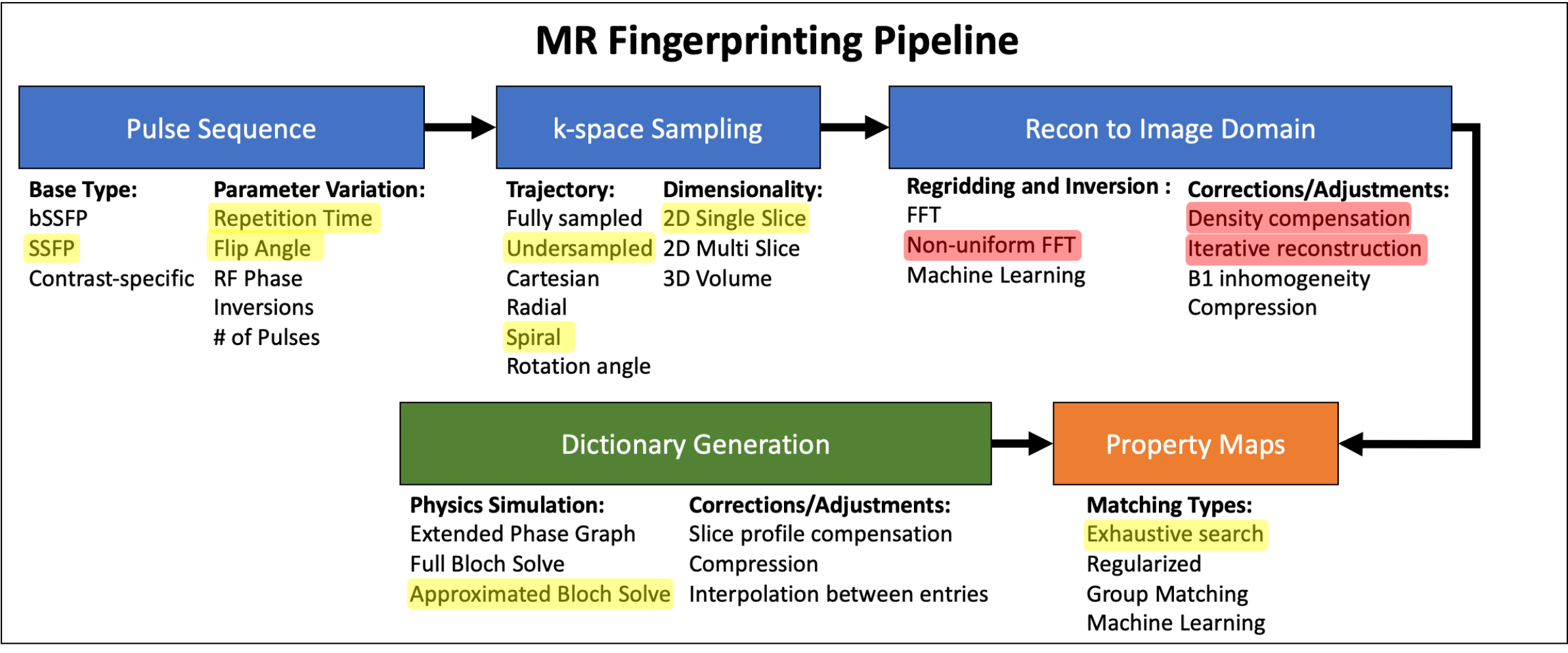
Figure 1: Overview of the MR Fingerprinting Pipeline.
The pipeline consists of acquisition (blue), dictionary generation (green), and property map creation (orange). At each stage of the pipeline there are many design choices that can be implemented, some of which are listed here. Each of these choices can influence the accuracy and precision of the resulting property maps. The design choices analyzed in this effort are highlighted in yellow (same across methods) and red (variable across methods).
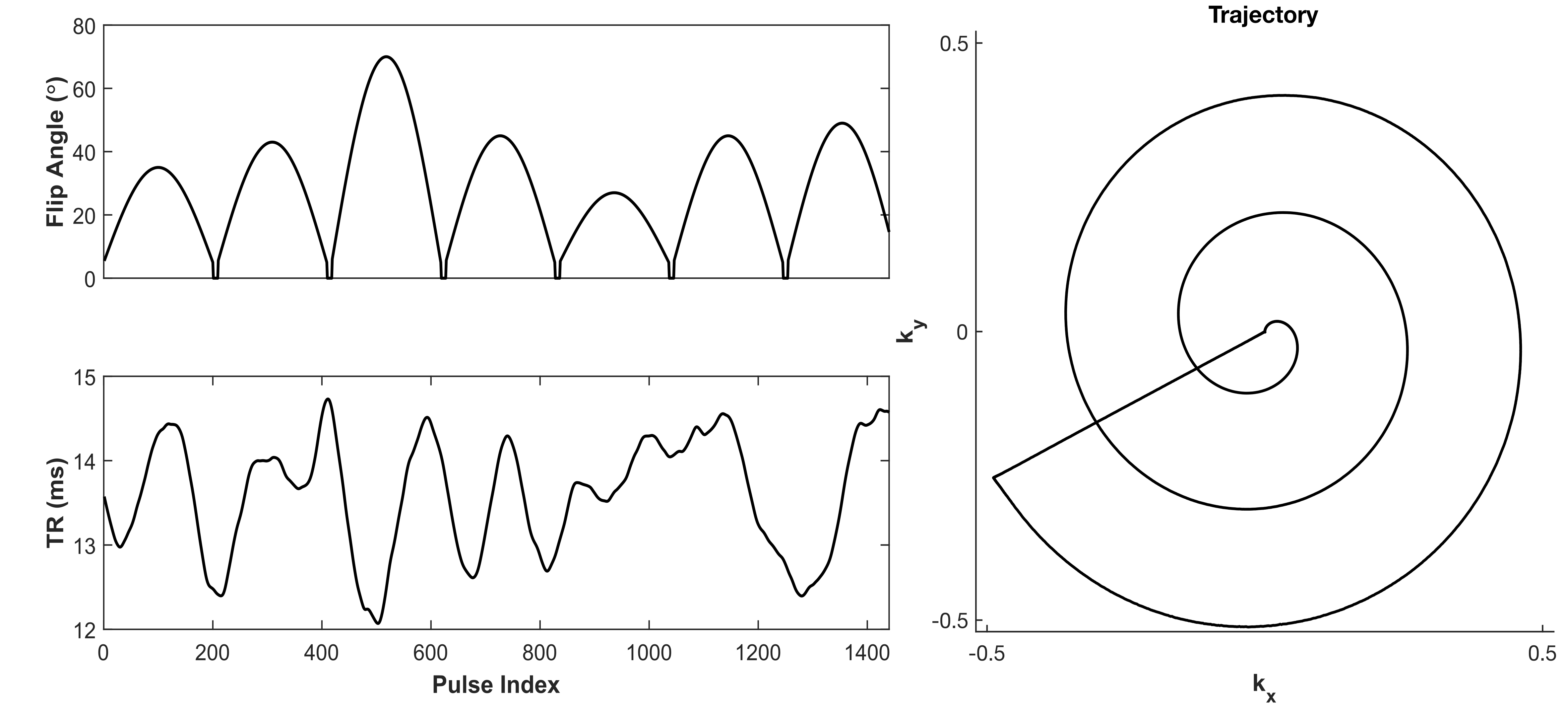
Figure 2: Pulse sequence used for data acquisition.
(A) Flip angle and repetition time (TR) pattern for the SSFP sequence that was used to acquire data. (B) Normalized, single arm k-space trajectory that was used to acquire data in k-space. For each subsequent RF pulse the trajectory was rotated 7.5 degrees. 2000 k-space points from each spiral were used in the reconstruction, eliminating the flyback to the center of k-space.
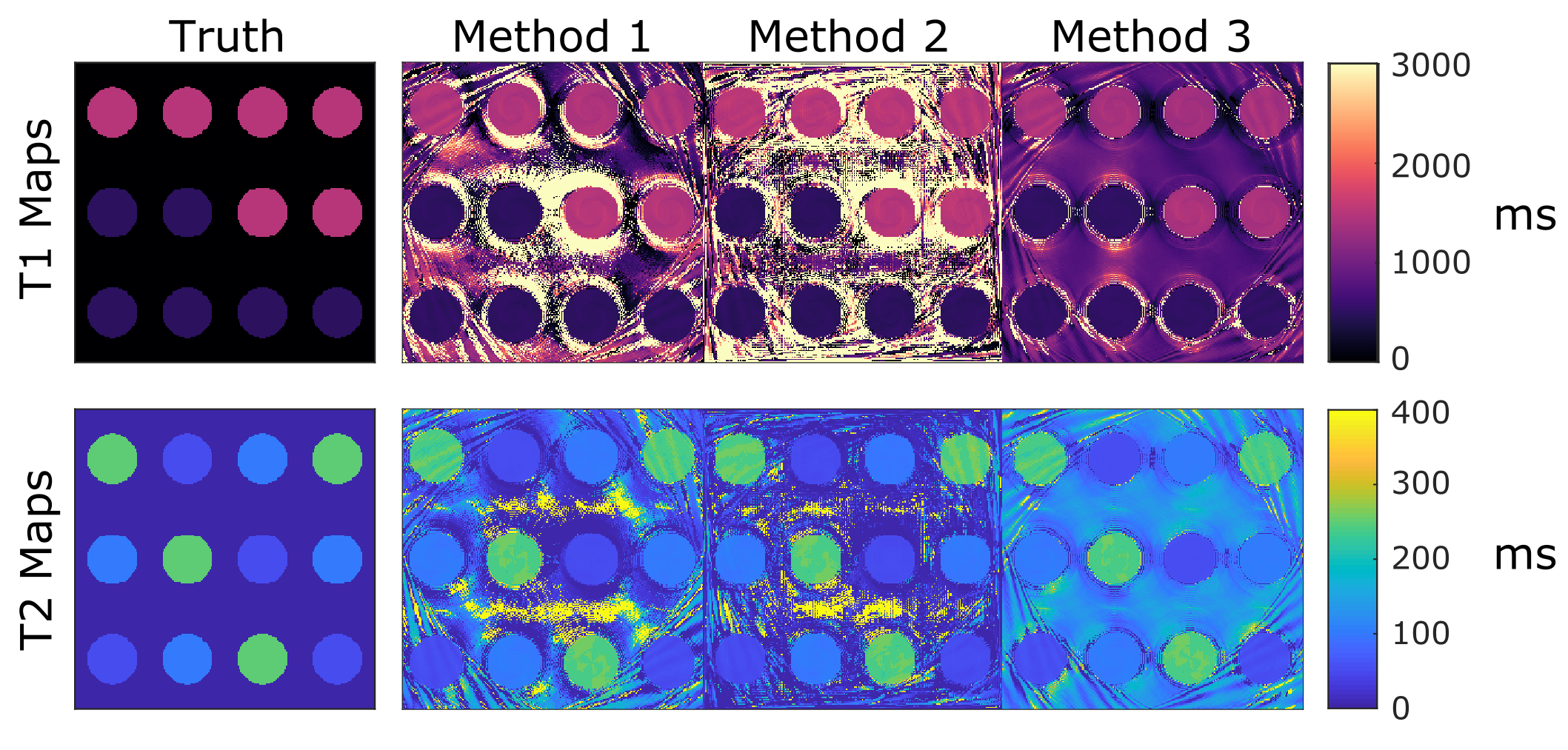
Figure 3: Simulated phantom reconstructed property maps for each method compared to the true values.
Qualitatively, the T1 and T2 maps generated with each method are in good agreement with the true values in the digital phantom. Spiral artifacts can be seen in the background where there is no signal, appearing stronger near the edges of the field of view where they begin to infiltrate the reconstructed maps within each circle.
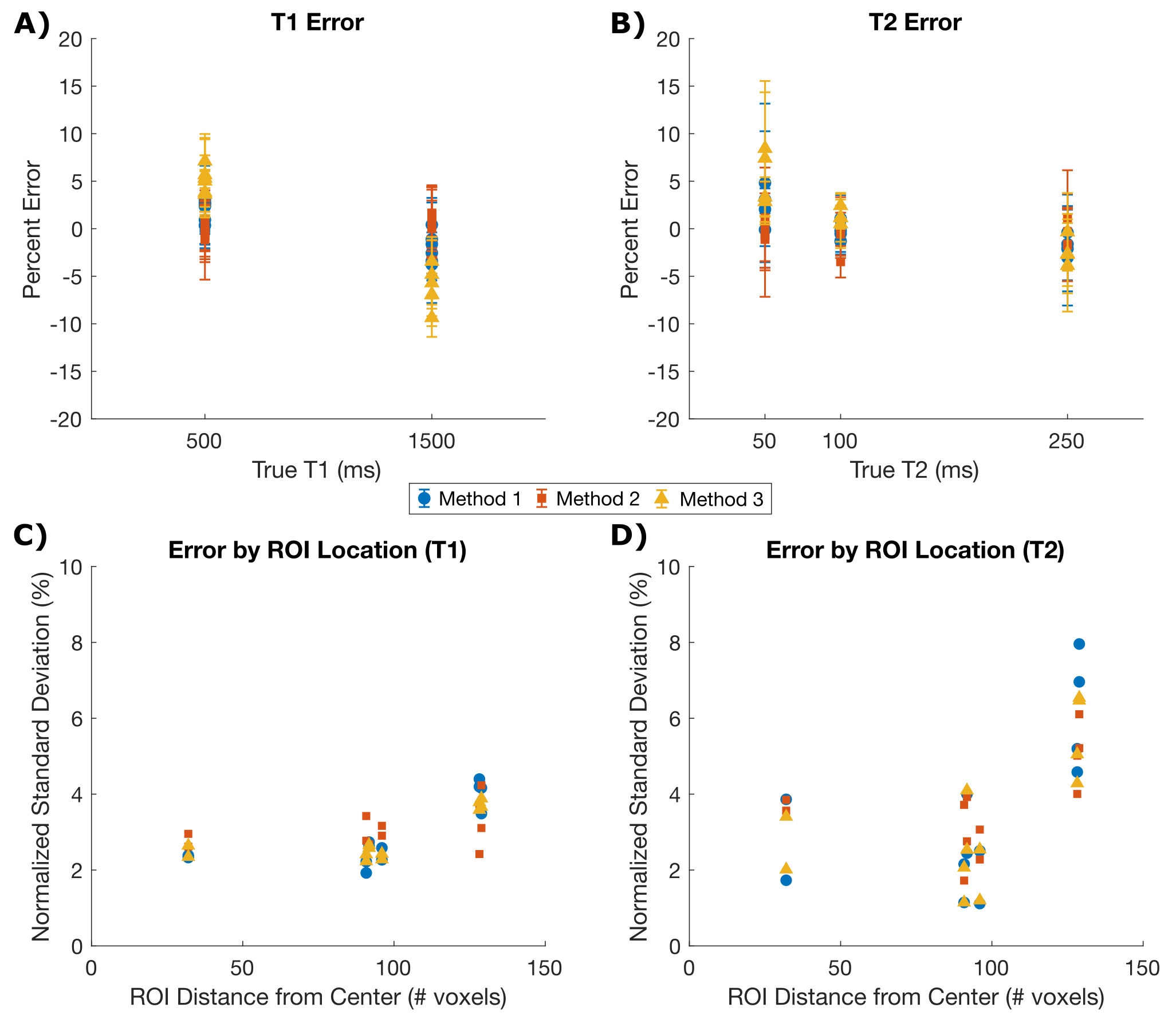
Figure 4: Simulated phantom quantitative analysis for each method.
Percent error from the true value within each circle of the digital phantom for T1 (A) and T2 (B). All methods result in less than 10% error with respect to the true value in each circle. Infiltration of artifacts near the edge of the phantom can be quantified by relating the ROI distance from the center of the FOV to the normalized T1 and T2 standard deviation for each circle (C and D).
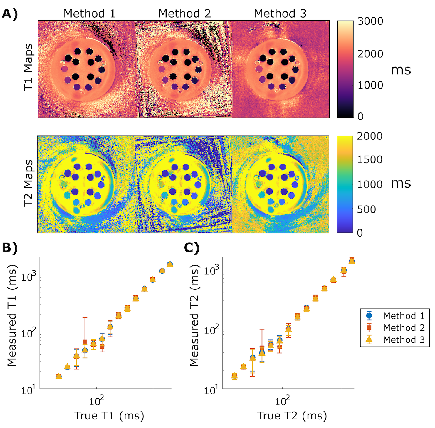
Figure 5: ISMRM/NIST phantom reconstruction results
(A) T1 and T2 maps generated of the NiCl2 array with the three non-uniform k-space reconstruction methods. All methods show similar property maps throughout the phantom and different artifact shapes outside the object. Qualitatively, Method 2 has more noise leakage into the maps.
(B and C) Mean T1 and T2 within each of the NiCl2 spheres from each reconstruction method plotted against the true T1 and T2 value. The error bars represent the standard deviation within each sphere.