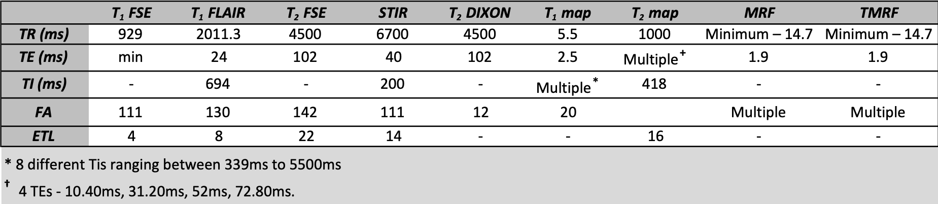
1548
A faster and improved tailored Magnetic Resonance Fingerprinting1Columbia Magnetic Resonance Research Center, Columbia University, New York, NY, United States, 2Dayananda Sagar College of Engineering, Bangalore, India
Synopsis
MR Fingerprinting (MRF) allows simultaneous acquisition of multi-parametric maps but the synthetic contrast images suffer from artifacts due to incomplete simulations. This work provides rapid (~4min), natural contrast (non-synthetic), quantitative (T1 and T2 maps), and qualitative images (T1-weighted, T1-FLAIR, T2-weighted, STIR, water,fat) simultaneously. Tailored MRF (TMRF) was demonstrated on four volunteers on 3T GE 750w scanner. It was compared with gold standard (GS) and MRF by computing SNR and mean intensity values of white matter (WM) and grey matter (GM) contrast. The SNR of GS>TMRF>MRF and the contrast for TMRF was greater than MRF and GS.
INTRODUCTION
Acquiring MR tissue parametric maps typically takes a longer time compared to qualitative MRI. MR fingerprinting (MRF)1 overcomes this with the simultaneous acquisition for multi-parametric maps. However, MRF has a limitation that it does not generate contrast images (routinely obtained in clinical scans). MRF reconstructed parametric maps are used to synthetically generate contrast images that are affected by incomplete simulations and system imperfections. Previously, we demonstrated tailored MRF (TMRF) that can (i) simultaneously acquire two tissue parametric maps and six non-synthetic qualitative MR contrasts in approximately 5.5 minutes for whole-brain coverage2. In this work, we have improved TMRF by (i) including two-point Dixon imaging (water and fat images); (ii) benchmarking with gold standard (GS) sequences; (iii) reducing scan time by 25%; (iv) reducing reconstruction time to less than two minutes; (v) deep learning (DL) based reconstruction for TMRF quantitative data (vi) TMRF image denoising using DL (vii) quantifying GM and WM signal intensities using 3D slicer software3; (viii) and comparing GS, MRF, and TMRF by computing SNRs and mean intensity values for GM and WM.METHODS
Water and fat contrasts were included by modifying the TE0 value of 1.9ms to 2.3ms and 3.4ms (TE1 and TE2 respectively). The in-phase and out-of-phase images were acquired and water and fat images were computed in MATLAB (The Mathworks Inc, MA). The GS protocol was set up on a 3T GE 750w scanner for the following sequences - T1 weighted, T1 FLAIR, T2 weighted, STIR, two-point Dixon for water and fat images, T1 and T2 mapping. Table 1 shows the acquisition details for all the GS sequences along with TMRF and MRF. Accelerated acquisition and reconstruction: TMRF was designed for specific combinations of repetition time (TR) and flip angle (FA), previously considering 1000 time points to yield 6 different contrasts. The time points for all 6 contrasts are within 575. The last block (750th to 1000) was discarded and only the first 749 time points were considered for the acquisition and this reduced the TMRF scan time by 25%. For image reconstruction using the sliding window, it previously took more than 40 minutes to reconstruct all the 1000 images. Currently, it takes 3 to 5 minutes, as the sliding window is applied only to six time points (corresponding to six contrasts) instead of all the time points. Quantitative maps: A DL based approach was used for TMRF in vivo quantitative map reconstruction. The network is a modified implementation of DRONE4 . Dictionary simulation was carried out using the same dictionary as in DRONE. The in vivo data was reconstructed offline without a sliding window using MATLAB and input to DRONE to obtain the quantitative maps. DL denoising: The SNR of few TMRF time points was lesser than GS due to incoherent noise and undersampled k-space. All the TMRF contrast images were denoised by learning the noise structure from the reconstructed images using the patches of noise obtained from TMRF images and forward modeled to train a Unet for denoising. The Human Connectome Project database was used to train and denoise the images while preserving the edges. The gradient anisotropic diffusion denoising method was used to remove the residual noise in slicer 3D. Image segmentation & SNR: 3D slicer5 was used to segment GM and WM for all 4 datasets. The segmentation was performed semi-automatically using the threshold method in the 3D slicer. SNR was computed for all the methods, across datasets using the “difference image” method. To compute the SNR, all the images were acquired twice under identical conditions. Besides, the mean contrast (difference between WM and GM) was calculated for all the three methods.RESULTS AND DISCUSSION
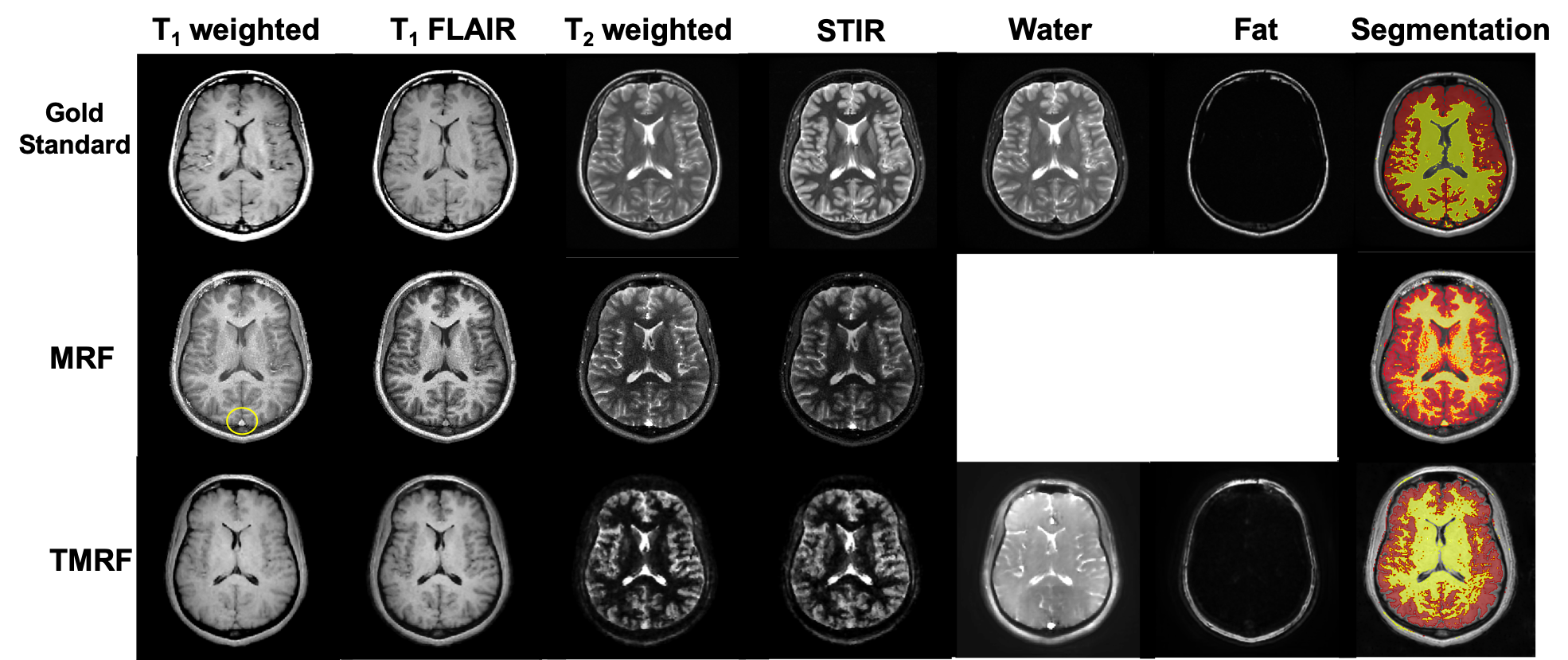
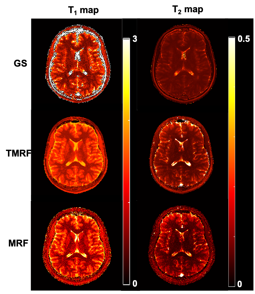
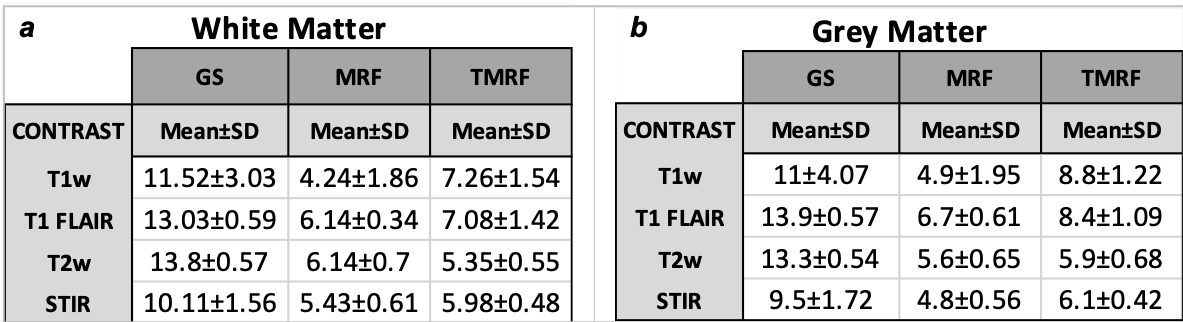
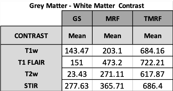
Figure 1 shows the qualitative healthy brain images using the GS method (first row), MRF (second row), and TMRF (third row). Each column represents different contrasts along with the representative GM and WM segmentation (last column) obtained using a 3D slicer. Images generated from MRF method were synthetically generated and flow artifacts are observed in all four contrasts (yellow circles). The flow artifacts can also be seen in water images obtained for TMRF. Figure 2 shows the in vivo brain quantitative images obtained from GS, TMRF, and MRF. GS T1 map was computed in Matlab and T2 map was obtained from GE software. Table 2 shows the SNR, computed using 3D slicer for all the three methods – GS, MRF and TMRF. Overall, the SNR of GS > TMRF > MRF. Table 3 shows the mean of means of WM and GM contrast values for all methods. The contrast was computed by taking the mean absolute differences between segmented GM and WM. It is observed that the TMRF GM/WM contrast is greater than GS and MRF. The total acquisition time for the GS sequences is ~23 minutes and TMRF provides all these contrasts along with two quantitative maps with the same resolution and number of slices in ~4 minutes whereas, MRF takes ~6 minutes to provide quantitative maps and synthetic images with artifacts and no Dixon imaging.CONCLUSION
TMRF provides a simpler and robust alternative to synthetic MRI approaches. Future work is to include diffusion-weighted imaging into TMRF design.Acknowledgements
This work was supported, in part, by GE-Columbia research partnership grant and also performed at Zuckerman Mind Brain Behavior Institute MRI Platform, a shared resource, and Columbia MR Research Center siteReferences
1. Ma D, Gulani V, Seiberlich N, Liu K, Sunshine JL, Duerk JL, Griswold MA, Magnetic resonance fingerprinting, Nature 2013
2. Pavan Poojar et. al., Natural, multi-contrast and quantitative imaging of the brain using tailored MR fingerprinting , ISMRM 2020.
3. http://www.slicer.org
4. Cohen, O., Zhu, B., & Rosen, M. S. (2018). MR fingerprinting Deep RecOnstruction NEtwork (DRONE). Magnetic Resonance in Medicine.
5. Pieper, S., Halle, M. and Kikinis, R., 2004, April. 3D Slicer. In 2004 2nd IEEE international symposium on biomedical imaging: nano to macro (IEEE Cat No. 04EX821) (pp. 632-635). IEEE.
Figures