1547
Myelin Water Imaging in the Hybrid State1Center for Biomedical Imaging, Department of Radiology, New York University School of Medicine, New York, NY, United States, 2Center for Advanced Imaging Innovation and Research, New York University School of Medicine, New York, NY, United States, 3Vilcek Institute of Graduate Biomedical Sciences, New York University School of Medicine, New York, NY, United States, 4Courant Institute of Mathematical Sciences, New York University, New York, NY, United States
Synopsis
This work extends the recently introduced hybrid-state model to myelin water imaging. We numerically optimize a hybrid-state MR fingerprinting sequence for SNR efficiency and demonstrate in vivo the ability to quantify the myelin water fraction and T2 of axonal/extra-axonal water. Our preliminary results show myelin water fraction maps in agreement with literature and demonstrate the feasibility of simultaneous myelin water fraction, T1 and T2 quantification with high spatial resolution (1.2mm isotropic), full brain coverage with a 14 minute scan.
Introduction
The gold standard in clinical imaging for multiple sclerosis (MS) has traditionally been fluid attenuation inversion recovery (FLAIR). However, hyperintensities in the FLAIR image are not specific and can be caused by different biophysical changes, including edema, inflammation, and demyelination[1]. Histopathological studies have demonstrated the utility of the myelin water fraction (MWF) and T2 of axonal/extra-axonal water ($$$T_2^s$$$; $$$s$$$ for slow) in distinguishing between inflammatory and demyelinating disease states[2].MR fingerprinting (MRF) triggered a wave research aimed at quantifying biomarkers in clinically feasible scan times. Prior work from our group introduced the hybrid-state[3], which provides improved SNR-efficiency compared to steady-state MR experiments[4]. This work extends the hybrid-state framework to a two compartment model. We optimize a pulse sequence for quantitative measurements of the MWF and T2s and demonstrate its performance in vivo in the human brain: we achieve a resolution of 1.2mm isotropic, whole brain in a 14min scan.
Theory
Assuming $$$T_R<<\{T_1,T_2\}$$$ and slow variations in the MRF sequence parameters, such as the flip angle, the dynamics of free spins can be captured by a radial component $$$r$$$ and a polar angle $$$\vartheta$$$ in spherical coordinates[3]. On-resonance, the polar angle is half the flip angle, which we assume in the following.We describe the signal in each voxel with an additive two-compartment model capturing the relaxation times of myelin water ("fast" relaxation) and axonal/extra-axonal water ("slow") while neglecting chemical exchange. This can be represented in the hybrid-state by the following system of ordinary differential equations
$$\partial{_t}\begin{bmatrix}r^f\\r^s\\1\end{bmatrix}=\begin{bmatrix}-\frac{\cos^2{\vartheta(t)}}{T^f_1}-\frac{\sin^2{\vartheta(t)}}{T^f_2}&0&\frac{f\cos{\vartheta(t)}}{T^f_1}\\0&-\frac{\cos^2{\vartheta(t)}}{T^s_1}-\frac{\sin^2{\vartheta(t)}}{T^s_2}&\frac{(1-f)\cos{\vartheta(t)}}{T^s_1}\\0&0&0\end{bmatrix}\begin{bmatrix}r^f\\r^s\\1\end{bmatrix},$$
where $$$\partial{_t}$$$ denotes the partial derivative with respect to time, $$$f$$$ is the MWF and the superscripts $$$^s$$$ and $$$^f$$$ denote the slow and fast compartments respectively. Then, the total measured signal $$$S$$$ in a voxel is simply $$$S(t)=M_0(r_f(t)+r_s(t))\sin\vartheta(t)$$$, where $$$M_0$$$ relates to the proton density.
Methods
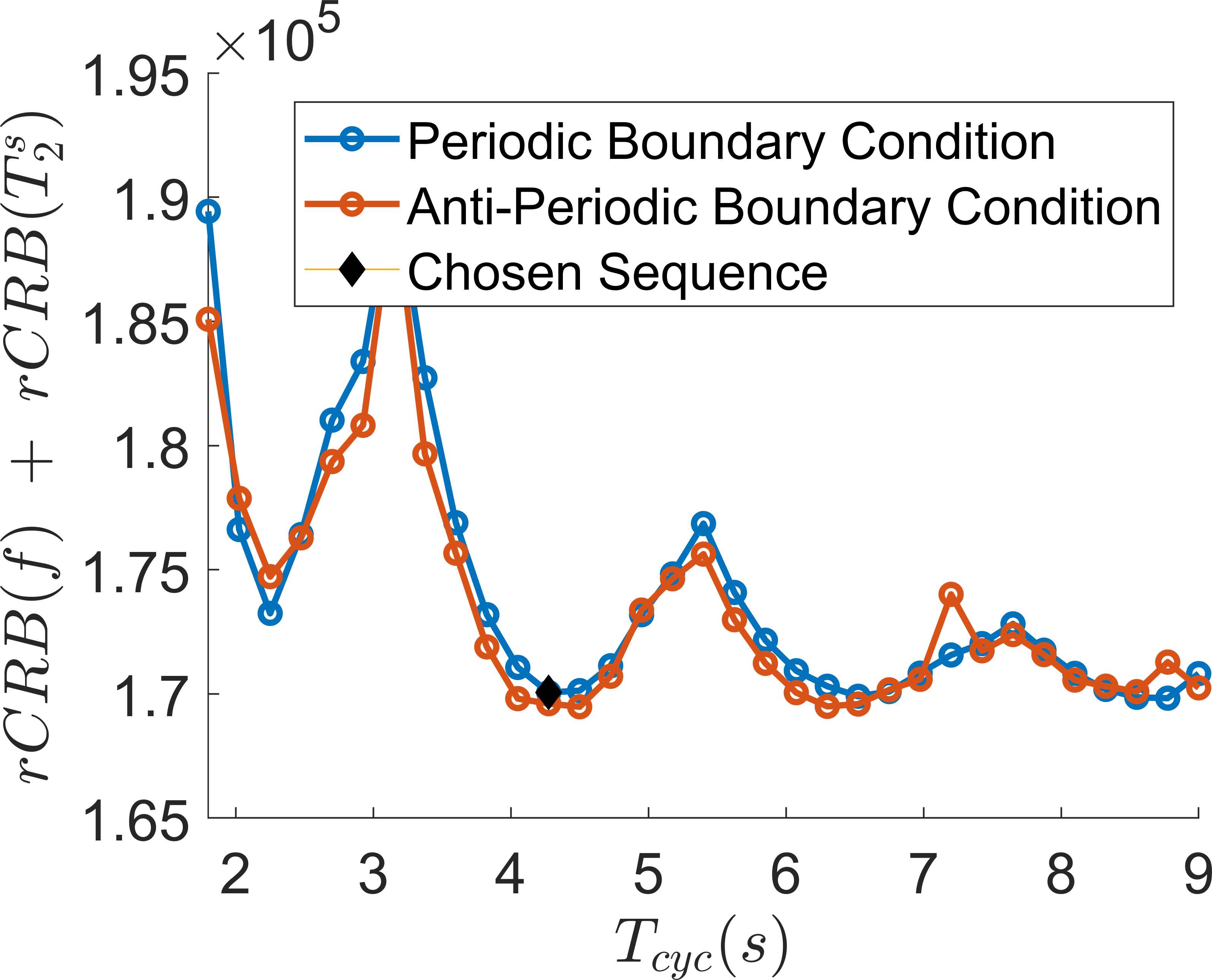
The above equation is solved using an ODE solver based on the Galerkin method[5]. To find the most SNR-efficient hybrid-state MRF sequence, we jointly calculate the relative Cramer-Rao bound (rCRB)[4] for $$$f$$$ and $$$T_2^s$$$ and minimize the sum numerically using the Broyden-Fletcher-Goldfarb-Shanno (BFGS) algorithm by optimizing $$$\vartheta$$$ as a function of time. We added a small $$$\ell_2$$$-norm total-variation regularization term to the cost function to prevent violations in the hybrid-state assumptions[3] and found that this does not significantly increase the rCRB. With a grid search, we further optimize the duration of a cycle $$$T_{cyc}$$$ and we repeat the cycles to fill the fixed scan time of 13.8min. We set $$$T_R=3.5$$$ms, limit $$$0\leq\vartheta\leq\pi/2$$$, and assume $$$T_1^s=1.1$$$s, $$$T_1^f=0.5$$$s[6] (slightly adjusted to account for acquisition at 3T), $$$T_2^s=65$$$ms, $$$T_2^f=10$$$ms and $$$f=0.11$$$[7]. We performed the optimizations for both periodic and anti-periodic boundary conditions[3].We tested the resulting sequence in vivo in an asymptomatic volunteer on a 3T Prisma scanner (Siemens, Erlangen, Germany). Spatial encoding was performed with a 3D golden angle koosh-ball trajectory[8]. The voxel size was $$$1.2$$$mm isotropic with an isotropic $$$FOV=230$$$mm.
We perform image reconstruction with BART[9] directly in a temporal subspace computed from a coarse dictionary[10],[11] and using locally low-rank regularization. Quantitative parameter maps are then calculated using non-linear least squares and a BFGS solver, with $$$T_1^f$$$ and $$$T_2^f$$$ fixed to literature values as their estimation is ill-conditioned. Spatial $$$B_1^+$$$ inhomogeneity is corrected by using an external $$$B_1^+$$$ measurement[12]. We scaled the map globally by a constant of $$$1.2$$$ to account for an anticipated underestimation.
Results and Discussion
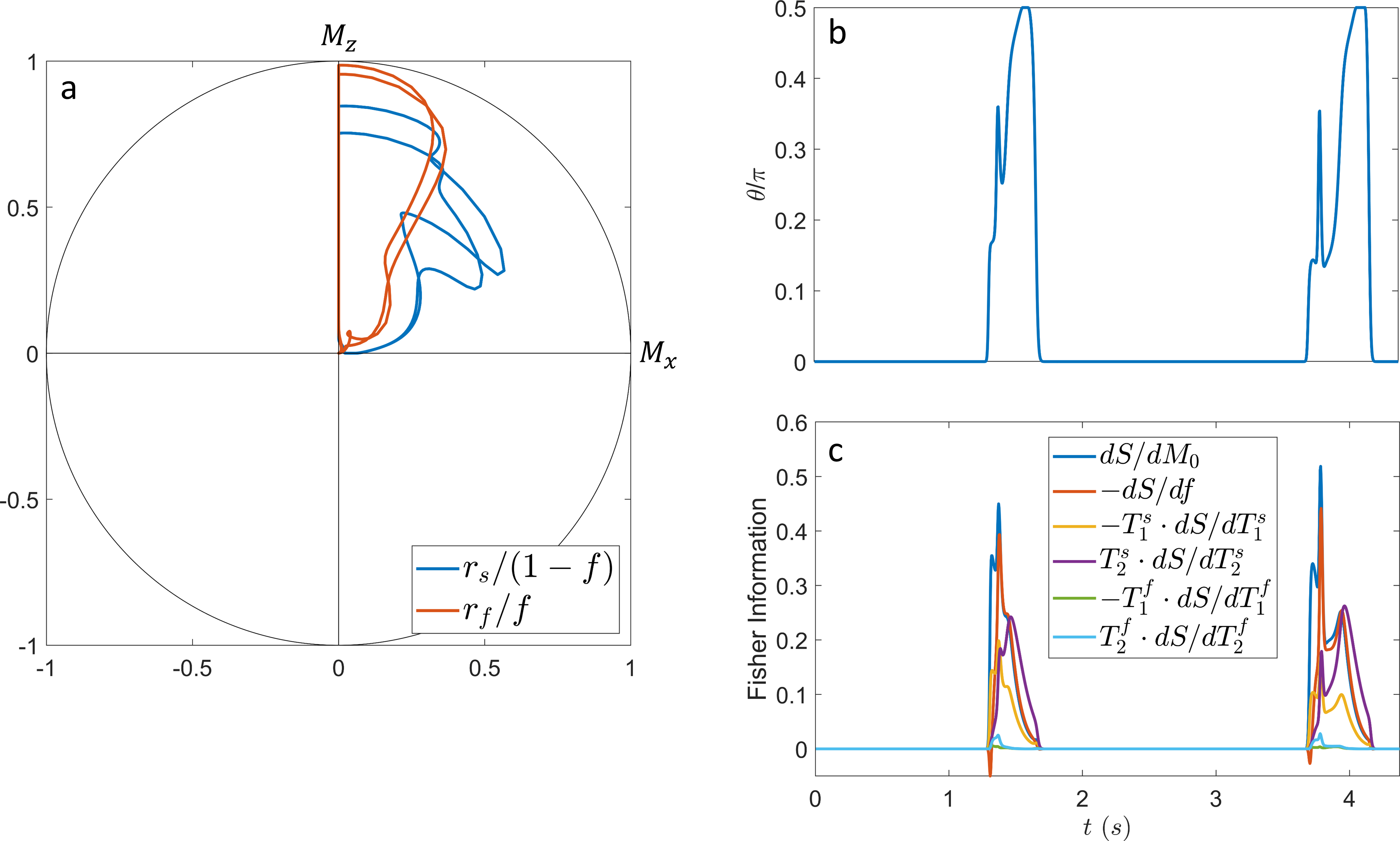
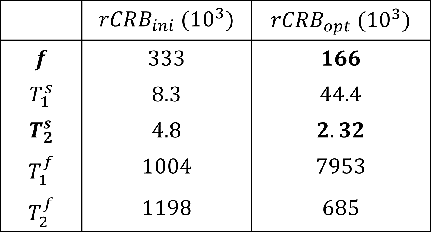
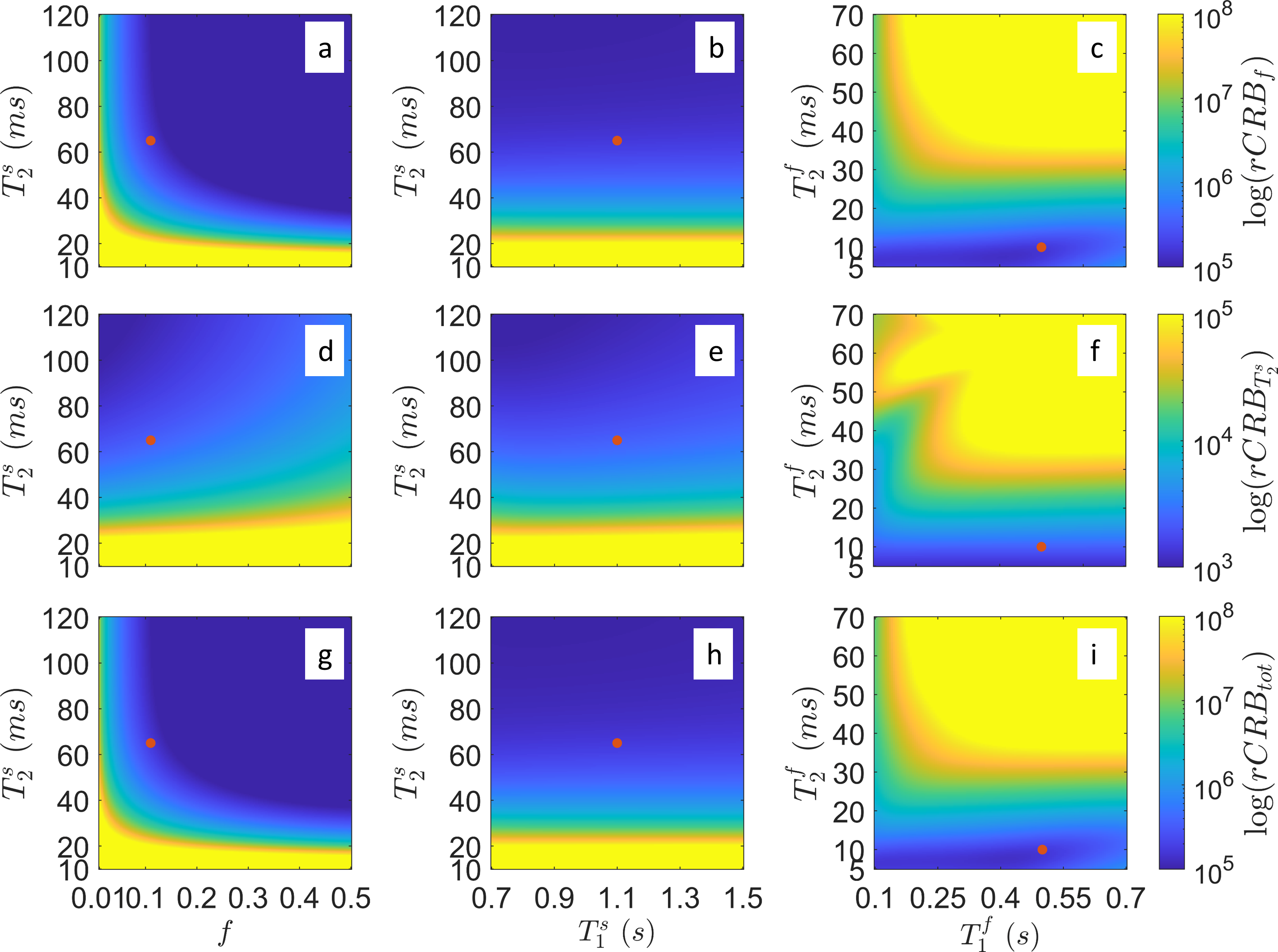
In contrast to our previous joint $$$T_1,T_2$$$ mapping approach[4], Figure 1 demonstrates that the optimized pulse sequences for anti-periodic and periodic boundary conditions have virtually equivalent performance. Since the inversion pulse predominantly encodes $$$T_1$$$, which is not optimized for here, the optimized anti-periodic pulse sequences simply apply the inversion pulse to a vanishing magnetization. Figure 2b shows the optimized pulse sequence with periodic boundary conditions. We observe that the optimization prefers a flip angle pattern that is zero for large portions of the sequence, instead maximizing the Fisher information, i.e. the gradient of signal with respect to the biophysical parameters, during two short periods of time, as shown in Figure 2c. The spin dynamics, shown in Figure 2a, demonstrate two loops that are limited to the northern hemisphere due to the missing inversion pulse.The rCRBs for the initial[4] and optimized sequence shown in Table 1 demonstrate a significant reduction in the Cramer-Rao bounds for $$$f$$$ and $$$T_2^s$$$. Figure 3 shows that these lower rCRB values are applicable to large areas of the parameter space.
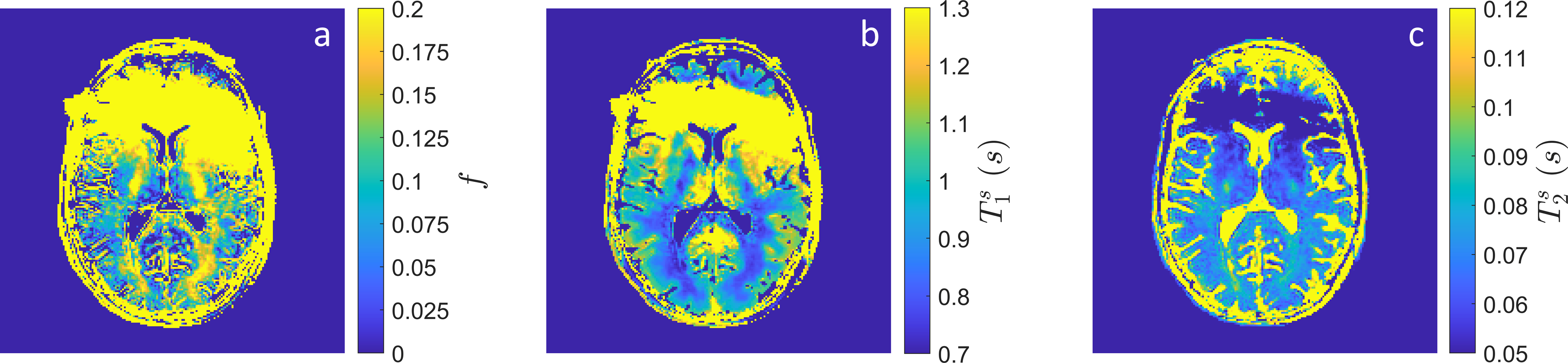
The in vivo parameter maps shown in Figure 4 demonstrate the feasibility for myelin water imaging in the hybrid-state. Several areas of white matter, including the posterior limb of the interior capsule, the corpus callosum splenium and forceps major, demonstrate increased MWF consistent with literature[13]. The anterior brain is unfortunately corrupted by a $$$B_0$$$ artifact resulting from metal in the volunteer's face mask.
For future work, we will seek to improve the $$$B_1^+$$$ mapping using the actual flip-angle approach[14] and include fast compartment parameters in our parameter fitting. We will also investigate the effect of chemical exchange, which can be readily incorporated in the above ODE, and perform a thorough in vivo comparison to established MWI methods, such as gradient-echo spin echo.
Acknowledgements
This work was supported by NIH grant R21 EB027241 and was performed under the rubric of the Center for Advanced Imaging Innovation and Research, a NIBIB Biomedical Technology Resource Center (NIH~P41 EB017183). A.M. is supported by NIH grant T32 GM136573.References
[1] Lee, J., Hyun, J. W., Lee, J., Choi, E. J., Shin, H. G., Min, K., … Oh, S. H. (2020). So You Want to Image Myelin Using MRI: An Overview and Practical Guide for Myelin Water Imaging. Journal of Magnetic Resonance Imaging, 1–14.
[2] Stanisz, G. J., Webb, S., Munro, C. A., Pun, T., & Midha, R. (2004). MR Properties of Excised Neural Tissue Following Experimentally Induced Inflammation. Magnetic Resonance in Medicine, 51(3), 473–479.
[3] Assländer, J., Novikov, D. S., Lattanzi, R., Sodickson, D. K., & Cloos, M. A. (2019). Hybrid-state free precession in nuclear magnetic resonance. Communications Physics, 2(1).
[4] Assländer, J., Lattanzi, R., Sodickson, D. K., & Cloos, M. A. (2019). Optimized quantification of spin relaxation times in the hybrid state. Magnetic Resonance in Medicine, 82(4), 1385–1397.
[5] Baccouch, M. (2016). The Discontinuous Galerkin Finite Element Method for Ordinary Differential Equations. In Perusal of the Finite Element Method. InTech.
[6] Stanisz, G. J., Kecojevic, A., Bronskill, M. J., & Henkelman, R. M. (1999). Characterizing white matter with magnetization transfer and T(2). Magnetic Resonance in Medicine, 42(6), 1128–1136.
[7] Laule, C., Vavasour, I. M., Moore, G. R. W., Oger, J., Li, D. K. B., Paty, D. W., & MacKay, A. L. (2004). Water content and myelin water fraction in multiple sclerosis: A T 2 relaxation study. Journal of Neurology, 251(3), 284–293.
[8] Chan, R. W., Ramsay, E. A., Cunningham, C. H., & Plewes, D. B. (2009). Temporal stability of adaptive 3D radial MRI using multidimensional golden means. Magnetic Resonance in Medicine, 61(2), 354–363.
[9] Ucker M, Ong F, Tamir JI, Bahri D, Virtue P, Cheng JY, et al., Bart: Version 0.2.09. Zenodo; 2015.
[10] Tamir, J. I., Uecker, M., Chen, W., Lai, P., Alley, M. T., Vasanawala, S. S., & Lustig, M. (2016). T 2 shuffling: Sharp, multicontrast, volumetric fast spin‐echo imaging. Magnetic Resonance in Medicine, 77(1), 180–195.
[11] Assländer, J., Cloos, M. A., Knoll, F., Sodickson, D. K., Hennig, J., & Lattanzi, R. (2018). Low rank alternating direction method of multipliers reconstruction for MR fingerprinting. Magnetic Resonance in Medicine, 79(1), 83–96.
[12] Chung, S., Kim, D., Breton, E., & Axel, L. (2010). Rapid B 1 + mapping using a preconditioning RF pulse with TurboFLASH readout. Magnetic Resonance in Medicine, 64(2), 439–446.
[13] Liu, H., Rubino, C., Dvorak, A. V., Jarrett, M., Ljungberg, E., Vavasour, I. M., Lee, L. E., Kolind, S. H., MacMillan, E. L., Traboulsee, A., Lang, D. J., Rauscher, A., Li, D. K. B., MacKay, A. L., Boyd, L. A., Kramer, J. L. K., & Laule, C. (2019). Myelin Water Atlas: A Template for Myelin Distribution in the Brain. Journal of Neuroimaging, 29(6), 699–706.
[14] Yarnykh, V. L. (2006). Actual flip-angle imaging in the pulsed steady state: A method for rapid three-dimensional mapping of the transmitted radiofrequency field. Magnetic Resonance in Medicine, 57(1), 192–200.
Figures