1546
High Accuracy Numerical Methods for Solving Magnetic Resonance Imaging Equations and Optimizing RF Pulse Sequences
Cem Gultekin1, Jakob Assländer2, and Carlos Fernandez-Granda3
1Mathematics, Courant Institute of Mathematical Science, New York, NY, United States, 2Radiology, New York University Grossman School of Medicine, New York, NY, United States, 3Mathematics and Data Science, Courant Institute of Mathematical Science and Center for Data Science New York University, New York, NY, United States
1Mathematics, Courant Institute of Mathematical Science, New York, NY, United States, 2Radiology, New York University Grossman School of Medicine, New York, NY, United States, 3Mathematics and Data Science, Courant Institute of Mathematical Science and Center for Data Science New York University, New York, NY, United States
Synopsis
This work presents a new robust black-box numerical solver that can reliably solve many MRI typical ordinary differential equations. Our adaptive Petrov-Galerkin (PG) method can solve challenging MRI problems with additional complexities such as B0- and B1- inhomogeneities, RF pulses, chemical exchange, and magnetization transfer (MT). We apply the proposed technique to solve an ODE-constrained optimization problem for pulse design via gradient descent. Our method reduces the time required to compute the gradients by three orders of magnitude.
Introduction
The design of pulse sequences, including for quantitative imaging, is commonly centered around a simple description of the underlying spin physics, such as exponential decays. Inspired by MR-Fingerprinting (MRF) 1 have been some efforts to trade model simplicity for a larger sequence design space in the search for improved encoding efficiency and/or accuracy 2,3,4,5. Here, we present a fast, high-precision solver tailored to the Bloch equation6 and its variations,such as the Bloch-McConnel equation7 which describes chemical exchange and magnetization transfer.Using PG, we find an efficient pulse sequence design by optimizing the RF pulses (i.e. the ”control”). Target of the optimization is to minimize the Cramer-Rao-Bound (CRB), which is a good predictor of the noise level in the estimated biophysical parameters. 2 Our pulse sequences are parameterized by individual flip-angles and pulse durations.
There are two numerical challenges behind optimal control of MRF experiments: first, we commonly want to optimize the flip angle of hundreds, or even over a thousand RF-pulses. Calculating the gradient with respect to each flip angle requires to solve a system of 3 x NRF-pulse differential equations, where we assume the simplest case of a standard Bloch simulation with three dimension (x,y,z). Second, RF-pulses create large abrupt changes in magnetization which creates instability for ODE solvers. With off-the-shelf ODE solvers, the computation time is prohibitively long. We propose here to use a Galerkin solver to overcome this issue.
Methods
Many MRI models can be put in the following form:$$$u'(t)=A(t)u(t)+b(t)$$$
Examples include Bloch equations, our hybrid-state model,2 exchanging and non-exchanging myelin-watermodels,8,9 as well as magnetization transfer.10 any quantitative MRI methods start at thermal equilibrium, and one commonly inserts gaps to allow return to thermal equilibrium before repeating the experiment for additional k-space lines. In order speed up the acquisition, we forgo these gaps. Mathematically, this turns the ODE into a linear boundary value problems (BVP) that relates the magnetization at the beginning and the end of each cycle2
$$$C_0u(0)+C_1u(T)=c.$$$
Here, u describes the magnetization dynamics throughout the experiment cycle of total duration T, and C are matrices with scaling parameters defining the boundary conditions. Further, we use the adjoint method11 which allows us to compute the gradients for any number of RF pulses by a single BVP solve.If we were to formulate our BVP problem as a concatenation of IVP problems, the calculation of the gradients has to go through all past iterations which effectively means a single IVP solve for each optimization parameter.
For such a large scale problem, speed requires adaptivity and Galerkin/spectral methods 12,13,14 are better at this than other BVP solvers such as collocation and multi-shooting. In Galerkin methods, a designated basis of test functions, v, enforces a discrete solution to satisfy the ODE by solving a linear system of equations seen as
$$$v(t)^Tu(t)\big|_{t_i}^{t_{i+1}}-\int_{t_i}^{t_{i+1}} (v'(t)+A(t)^Tv(t))^Tu(t)dt=\int_{t_i}^{t_{i+1}}v(t)^Tb(t)dt$$$
Petrov-Galerkin methods design test functions tailored for each class of problem 15. Our test space choice is approximate solutions to local adjoint differential problem. For f chosen from a polynomial basis, such test functions solve
$$$v'(t)+A(t)^Tv(t)\approx f(t),\quad t \in [t_i,t_{i+1}]$$$
By putting more effort on solving easier smaller local problems, higher rate of convergence can be achieved without increasing number of unknowns. This is critical for performance of PG as the number of unknowns while solving MRI BVP grows rapidly.
Results and Discussion
As an example of application, we optimized a pulse sequence for quantitative MT with a hybrid-state model 16. Given a fixed TR=3.5 msec, we optimized pulse sequences with cycle duration T between 1 to 6 seconds and found the lowest CRB for T = 4 sec. This equates to an optimization with around 2,200 parameters. The optimization duration of this scale varied around 5 to 7 hours, while it would unfeasible with off-the-shelf IVP methods. This advantage of our PG approach is highlighted by error-over-time plot in Fig. 3. Fig. 4 shows that the computation time is virtually constant when increasing the optimization dimension, i.e. the number of RF-pulses in our case. Figure 5 demonstrates the feasibility of our solver for fitting the MT model to in vivo data.Acknowledgements
This work was supported by NIH grant R21 EB027241 and was performed under the rubric of the Center for Advanced Imaging Innovation and Research, a NIBIB Biomedical Technology Resource Center (NIH~P41 EB017183).References
- Dan Ma et al. “Magnetic resonance fingerprinting”. In: Nature495. 7440(2013), pp. 187–192. issn: 0028-0836
- Jakob Asslander et al. “Hybrid-state free precession in nuclear magnetic resonance”. In: Nat. Commun. Phys. 2.1 (2019), p. 73. issn: 2399-3650.
- Jakob Asslander et al. “Optimized quantification of spin relaxation times in the hybrid state”. In: Magn. Reson. Med.82.4 (2019), pp. 1385–1397. issn: 0740-3194. doi:10.1002/mrm.27819. arXiv:1703.00481.
- Bo Zhao et al. “Optimal Experiment Design for Magnetic Resonance Fingerprinting: Cramér-Rao Bound Meets Spin Dynamics”. In:IEEE Trans.Med. Imaging 38.3 (2019), pp. 844–861.
- Jakob Asslander. “A Perspective on MR Fingerprinting”. In: J. Magn. Reson. Imaging(2020). issn: 10531807. doi:10.1002/jmri.27134.
- F. Bloch. “Nuclear induction”. In:Phys. Rev.70.7-8 (1946), pp. 460–474.
- Harden M. McConnell. “Reaction Rates by Nuclear Magnetic Resonance”. In: J. Chem. Phys.28.3 (1958), pp. 430–431.
- Alex Mackay et al. “In vivo visualization of myelin water in brain by magnetic resonance”. In: Magn. Reson. Med.31.6 (1994), pp. 673–677.
- C. Laule et al. “Water content and myelin water fraction in multiple sclerosis: A T2 relaxation study”. In:J. Neurol.251.3 (2004), pp. 284–293.
- RM M Henkelman et al. “Quantitative Interpretation of Magnetization Transfer”. In: Magn. Reson. Med. 29.6 (1993), pp. 759–766
- Lorenz T Biegler et al. “Large-scale PDE-constrained optimization: an introduction”. In: Large-Scale PDE-Constrained Optimization. Springer, 2003, pp. 3–13.
- Anders Logg. “Multi-adaptive Galerkin methods for ODEs I”. In: SIAM Journal on Scientific Computing24.6 (2003), pp. 1879–1902.
- Slimane Adjerid and Mahboub Baccouch. “The discontinuous Galerkinmethod for two-dimensional hyperbolic problems. Part I: Superconver-gence error analysis”. In: Journal of Scientific Computing 33.1 (2007), pp. 75–113.
- June-Yub Lee and Leslie Greengard. “A fast adaptive numerical method for stiff two-point boundary value problems”. In: SIAM Journal on Scientific Computing 18.2 (1997), pp. 403–429.
- Albert Cohen, Wolfgang Dahmen, and Gerrit Welper. “Adaptivity andvariational stabilization for convection-diffusion equations”. In: ESAIM: Mathematical Modelling and Numerical Analysis 46.5 (2012), pp. 1247–1273.
- Jakob Assl ̈ander and Daniel K Sodickson. “Quantitative Magnetization Transfer Imaging in the Hybrid State”. In: Proc. Intl. Soc. Mag. Reson. Med. 27. 2019, p. 1104.
Figures
Optimization result acquired with PG on
Hybrid-State model. Targeted relative CRB values after minimization
rCRB(m0s)=1.1 · 10^5, rCRB(T1)=2.0 · 104 and rCRB(T2f)=3.26 ·104.
Biophysical parameters included in the CRB computation are proton
density=1, m0s=0.1, T1=1.6 sec, T2f=65 msec, R=30, T2s=60 µsec, B0 and B1. Relative CRB is defined as rCRB(T1)=CRB(T1)Texp/TRT12
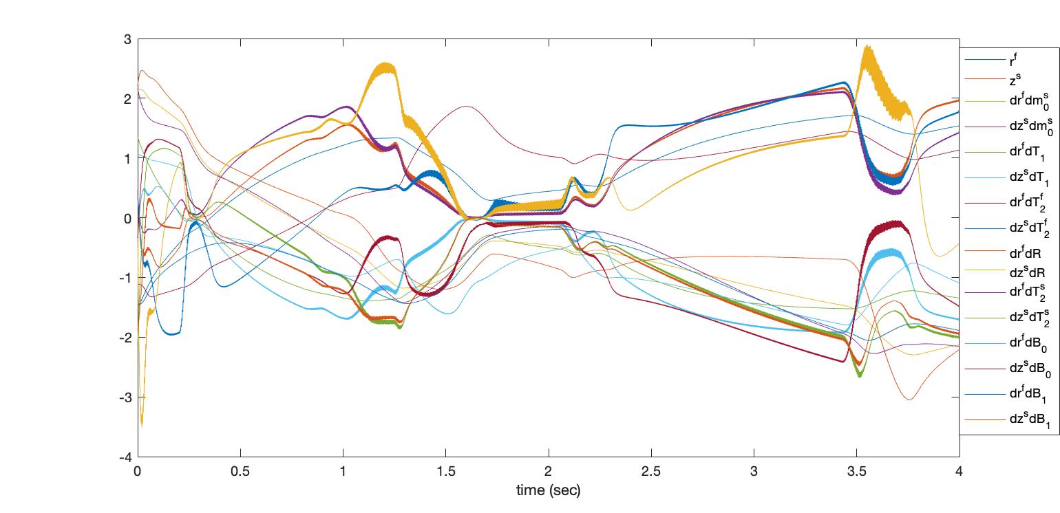
Hybrid-State equations solved by PG for cycle of 4 seconds. Each signal is normalized by its mean magnitude for visualization. The oscillations are aligned with RF pulses. Representation of such a signal by piece-wise polynomials needs higher orders which quickly blows up the number of unknowns to solve the BVP. PG can increase order of accuracy without increasing the number of unknowns by putting more effort to locally defined simple problems.
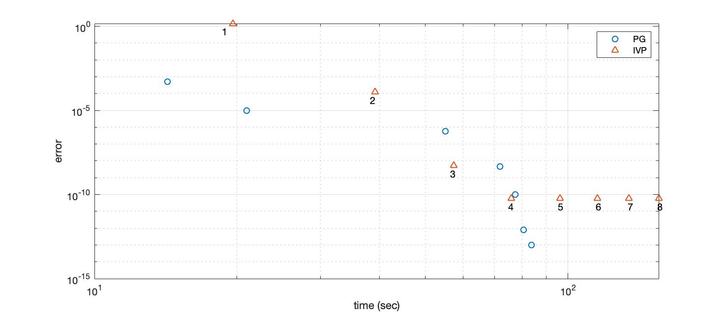
We used MATLAB's ode45 method to solve repeated IVP cycles of Hybrid-State model, a total of 8 iterations. Number underneath the points for IVP stand for iteration number. PG achieves comparable performance to IVP in simulation time. This is including error control and adaptation steps of PG.
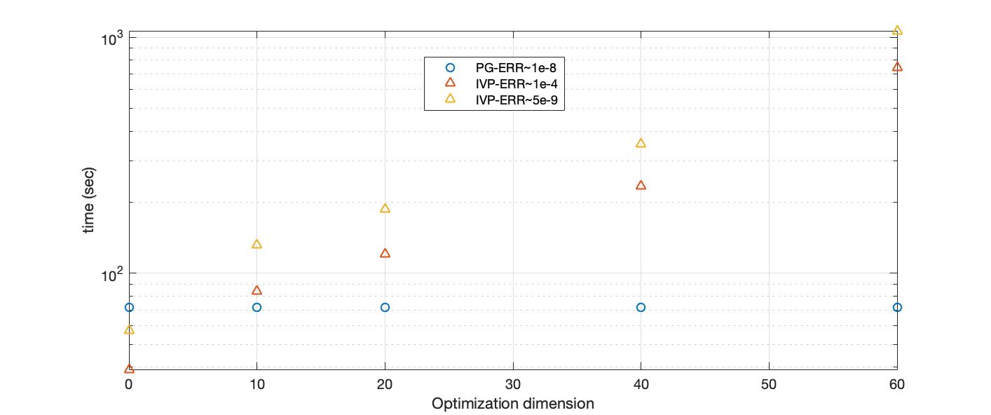
For IVP solvers, it gets unfeasible quickly to have higher dimensional optimization. However, with BVP formulation, the dimension does not impact the simulation time.
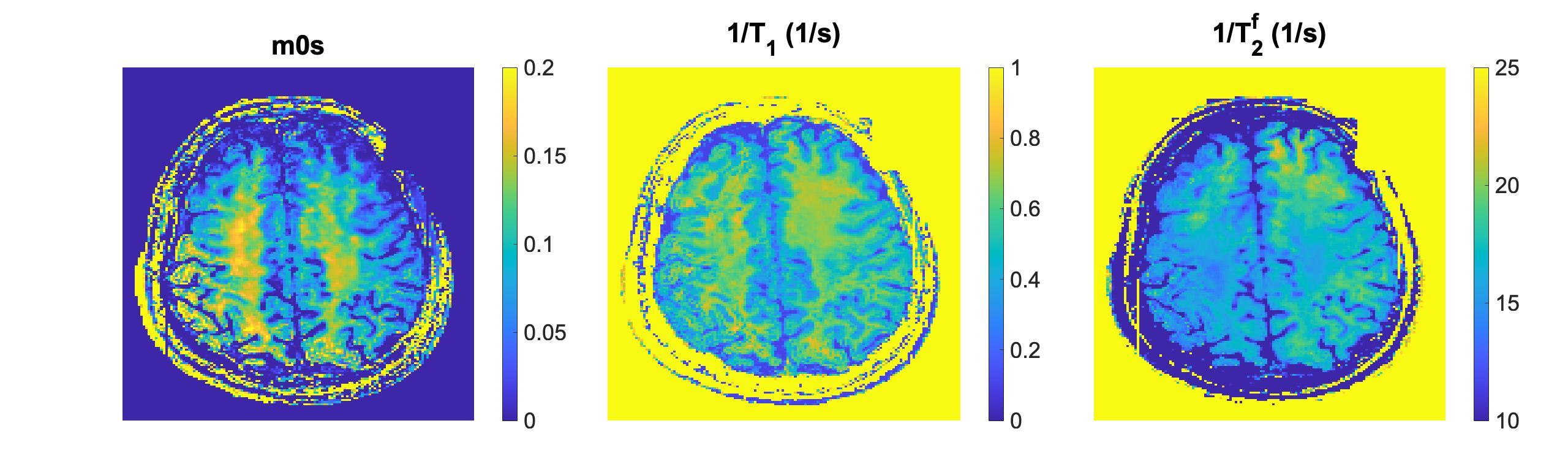
The in vivo data parameter maps demonstrate the utility of the PG solver for non-linear-least square fitting. Here, we use a hybrid state MT model as an example and show the semi-solid spin-pool fraction (m0s), an apparent T1 relaxation time, and the T2f relaxation time of the free pool.