1543
Estimating tissue volume fractions and proton density in multi-component MRF1Department of Imaging Physics, Delft University of Technology, Delft, Netherlands, 2Department of Radiology and Nuclear Medicine, Erasmus MC, Rotterdam, Netherlands, 3C.J. Gorter Center for high field MRI, Department of Radiology, Leiden University Medical Center, Leiden, Netherlands, 4Department of Radiology, Leiden University Medical Center, Leiden, Netherlands
Synopsis
Accurate proton density estimations are required to obtain tissue volume fractions from multi-component MR Fingerprinting data. We propose a method for estimating relative proton densities per tissue while taking the receiver sensitivity profile into account. In 20 different numerical brain phantoms this shows to improve tissue segmentations compared to conventional methods that use $$$T_1$$$ weighted images. Estimated proton density values for single slice in vivo data (7 scans for 4 subjects) were in range with literature values in particular for white and gray matter.
Introduction
Brain volume is an imaging marker that is often affected in neurodegenerative diseases, e.g. Alzheimer’s disease[1]. Therefore, accurate measurement of brain tissue volumes is important for diagnostic and prognostic studies and potentially also for treatment studies. For multi-site studies, highly robust brain volume measurements are particularly needed[2].Correct estimations of partial volume in tissue segmentations can provide more insight into subtle structural changes and are indispensable for correct voxel-wise comparisons[3]. Quantitative MR methods such as MR fingerprinting(MRF)[4] hold the promise to improve robustness, repeatability and reproducibility of the measurements[5]–[7].
Multi-component MRF using joint sparsity constraints allows estimation of tissue fractions based on the tissue magnetization per voxel by identifying the different $$$T_1$$$-$$$T_2$$$-signal characteristics[8]. However, this approach overestimates the fraction of high proton density(PD) tissues, which may lead to an underestimation of especially white matter volumes.
We propose a new method to determine PD per tissue based on estimated tissue magnetization maps from MC-MRF, resulting in quantitative tissue volume fraction maps. In simulations these estimations are compared to segmentations of $$$T_1$$$-weighted images. Furthermore, in vivo reproducibility of MC-MRF estimations is verified.
Theory
Multi-component MRF describes reconstructed signal evolutions $$$X\in\mathbb{R}^{t\times J}$$$($$$t$$$ time points, $$$J$$$ voxels) as linear combination of signals $$$d_i=S(T_1^i,T_2^i)\in\mathbb{R}^t$$$, simulated with $$$PD=1$$$, and effective magnetization per tissue component $$$M_i\in\mathbb{R}^J$$$. Practically, tissue magnetization results from a combination of PD $$$d_i$$$, volume fraction $$$F_i\in\mathbb{R}^J$$$, voxel volume $$$v$$$ and a combined receive coil $$$B_1^-$$$-field $$$R\in\mathbb{R}^J$$$.[9]In a two-fold approach we first calculate$$\hat{M}=\text{argmin}_{\widetilde{M}\in R_{\geq~0}^{N\times J}}\left\lVert~X-D\tilde{M}\right\rVert_F+\mu \sum_{i=1}^N\left\lVert \tilde{M}_i\right \rVert _0$$using the SPIJN algorithm[8], where $$$D=\left[d_1,\ldots,d_N\right]$$$ and $$$\hat{M}=\left[{\hat{M}}_1^T,\ldots,\ {\hat{M}}_N^T\right]^T$$$. This problem consists of a data fidelity term and a joint sparsity term regularized by $$$\mu$$$, enforcing a small number of tissues. Only non-zero maps ($$$\left\lVert \tilde{M}_i\right\rVert>0$$$) are saved and reindexed, as $$$\left[M_1^T,\ldots,\ M_K^T\right]=M\in\mathbb{R}^{K\times J}$$$.
In a second step $$$M_i$$$ is factorized as$$M_i=R\circ~F_i\cdot~d_i\cdot~v,$$$$$R$$$ is modelled as smoothly varying[9] through a 2D/3D polynomial parametrized by $$$\mathbf{p}\in\mathbb{R}^P$$$. Assuming$$$~\sum_{i}\ F_i=\mathbf{1},~$$$the following holds:$$\frac{M_i}{d_i}=R\left({\mathbf{p}}\right)\circ\ F_i\cdot\ v,$$$$\sum_{i}{M_i/d_i}=\sum_{i}{R({\mathbf{p}})\circ F_i\cdot v},$$$$\sum_i~\frac{M_i}{d_i}=vR(\mathbf{p}).$$
Methods
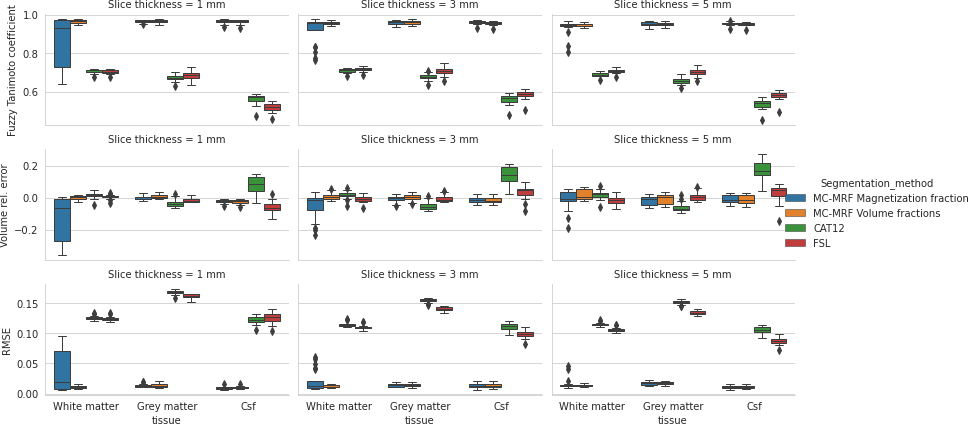
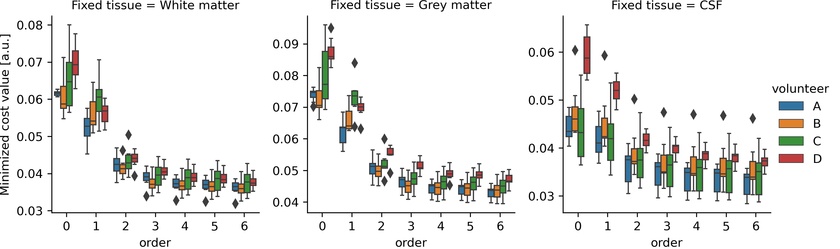
The minimization problem$$\text{argmin}_{\mathbf{d}\in\mathbb{R}_{\geq0}^K,~\mathbf{p}\in\mathbb{R}^P}\left\lVert\rho\left(\sum_{i}\frac{M_i}{d_i}-vR\left(\mathbf{p}\right)\right)\right\rVert_2^2$$is solved using a robust least squares solver applying $$$\rho(z)=2(\sqrt{1+z^2}-1)$$$, i.e. an $$$L_1$$$-approximation, to estimate PDs and $$$R$$$, from which volume fractions $$$F_i$$$ are obtained. To avoid the trivial solution $$$\mathbf{p}=\mathbf{0},\mathbf{d}=\mathbf{0}$$$, the relative PD is calculated with respect to a “fixed” tissue $$$j$$$, enforced by setting $$$d_j=1$$$(gray matter was used for shown results).20 BrainWeb numerical phantoms[10] (with RF-distortion field ‘C’) were used to determine partial volume tissue estimates using SIENAX-FSL[11], SPM12-CAT[12] and MC-MRF(our approach). Tissue segmentations were compared to ground truth values regarding the relative error in total volume, the normalized root mean squared error (NRMSE) and a continuous Dice’s coefficient, the fuzzy Tanimoto coefficient ($$$FC_F\left(X,Y\right)=\frac{\sum\min\left(X,Y\right)}{\sum\max\left(X,Y\right)}$$$)[13].
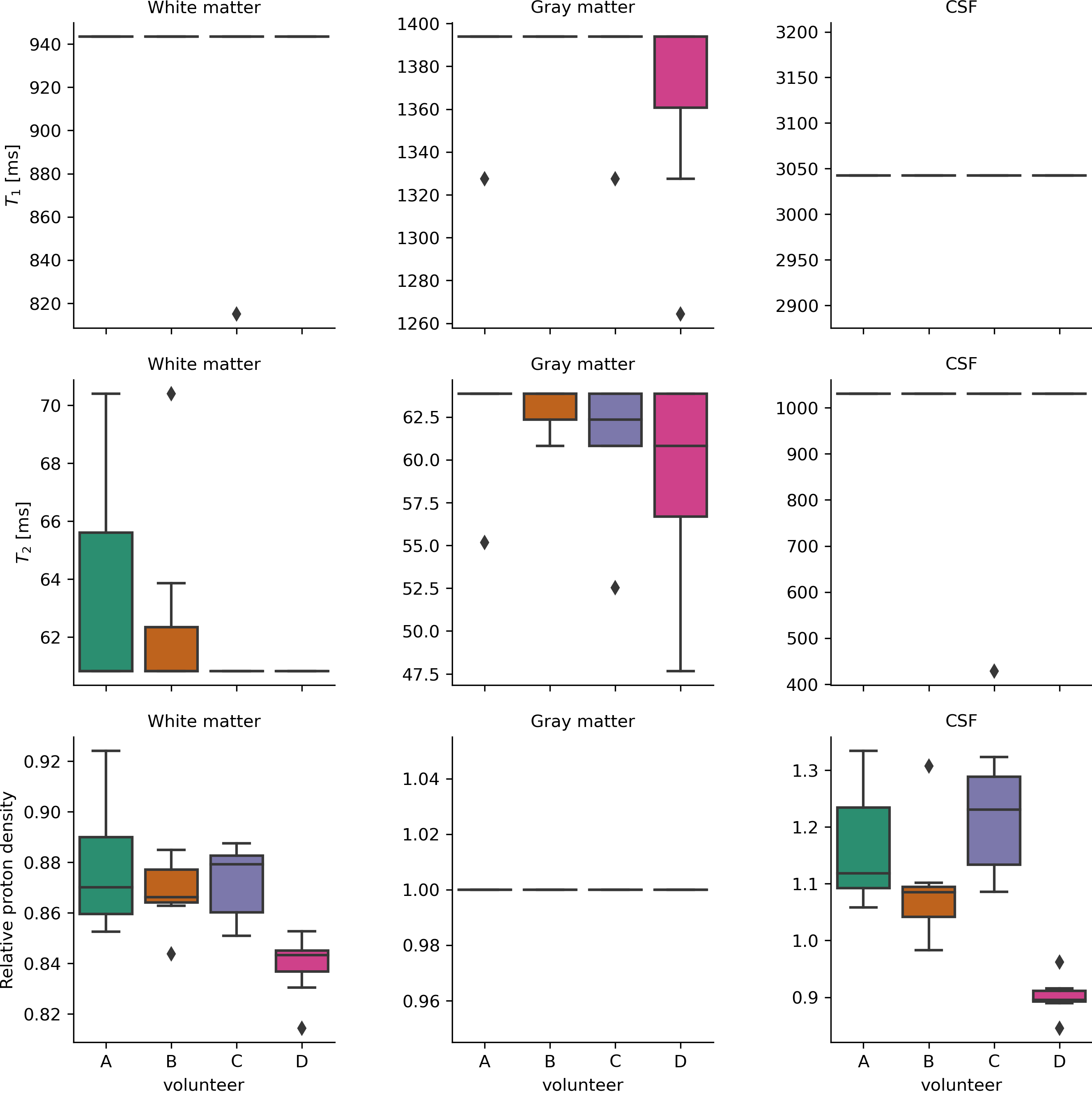
Retrospective analysis was performed on FISP-MRF data[4]. Data was acquired with a 3.0T scanner(GE MR70)(FOV=31x31cm2,voxel size=1.2x1.2x5 mm3). 4 volunteers were scanned 7 times for 7 consecutive weeks. Single slice data was analysed. Multi-slice data of one volunteer was used as reference data.
Results
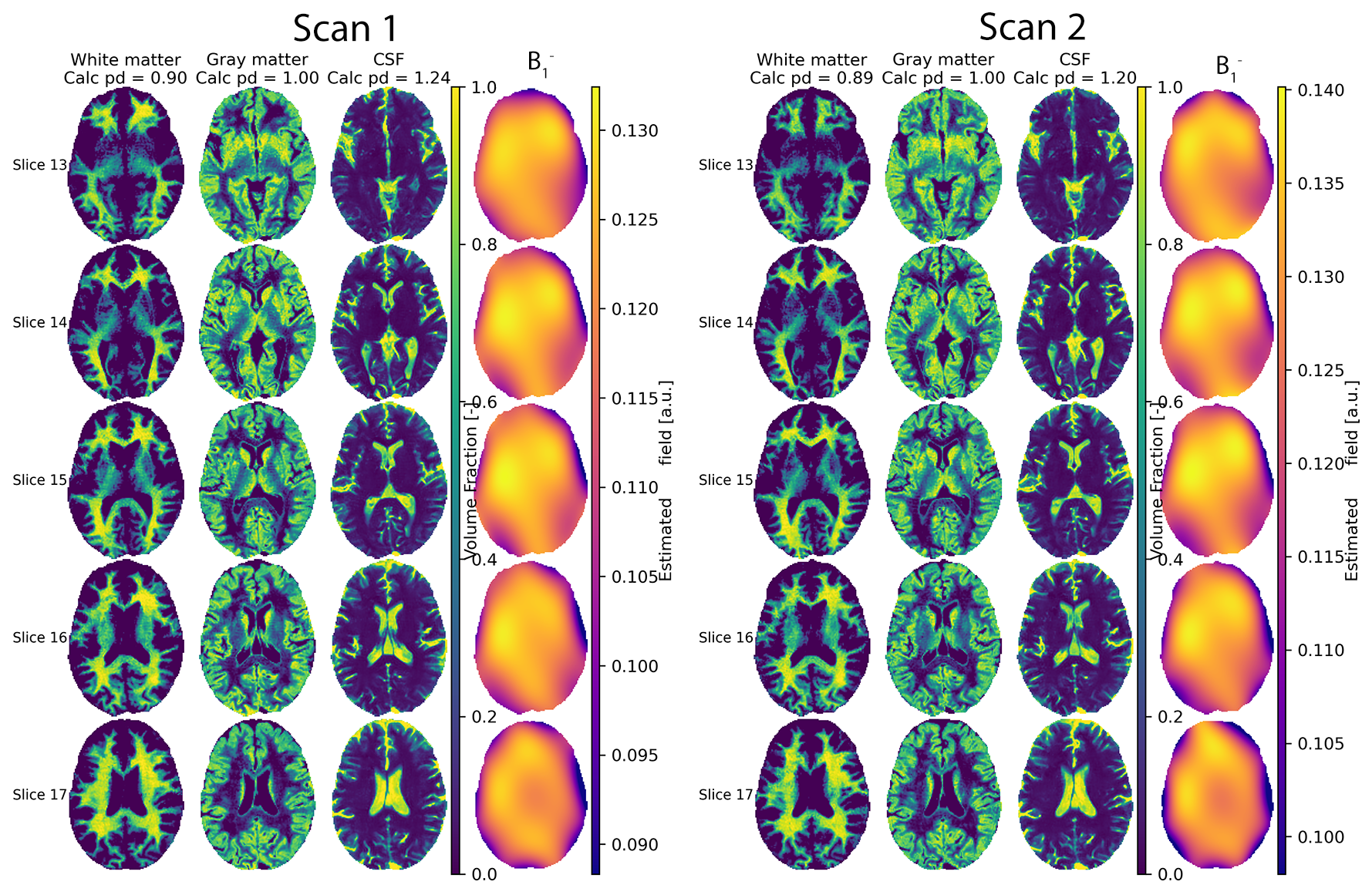
The simulations demonstrated that the proposed method was able to accurately estimate the PDs and volume fraction maps across all tissues and metrics(Fig.1). Comparison between the ‘uncorrected’ magnetization fractions and ground truth volume fractions demonstrates the anticipated systematic errors (especially for WM resulting in large volume errors). The T1w-based methods give accurate volume estimations, but larger errors in RMSE and $$$TC_F$$$, especially for CSF and increasingly so for thicker slices (also in volume error).In vivo data was processed with different polynomial orders and fixed tissue PD, yielding stable solutions for order$$$\geq~3$$$, irrespective of the fixated tissue(Fig.2). Estimated PD values were in line with literature[14](Fig.3), but PD of CSF showed more variation. Estimated relaxation times were very similar across scans, but GM showed lower values than literature[15].
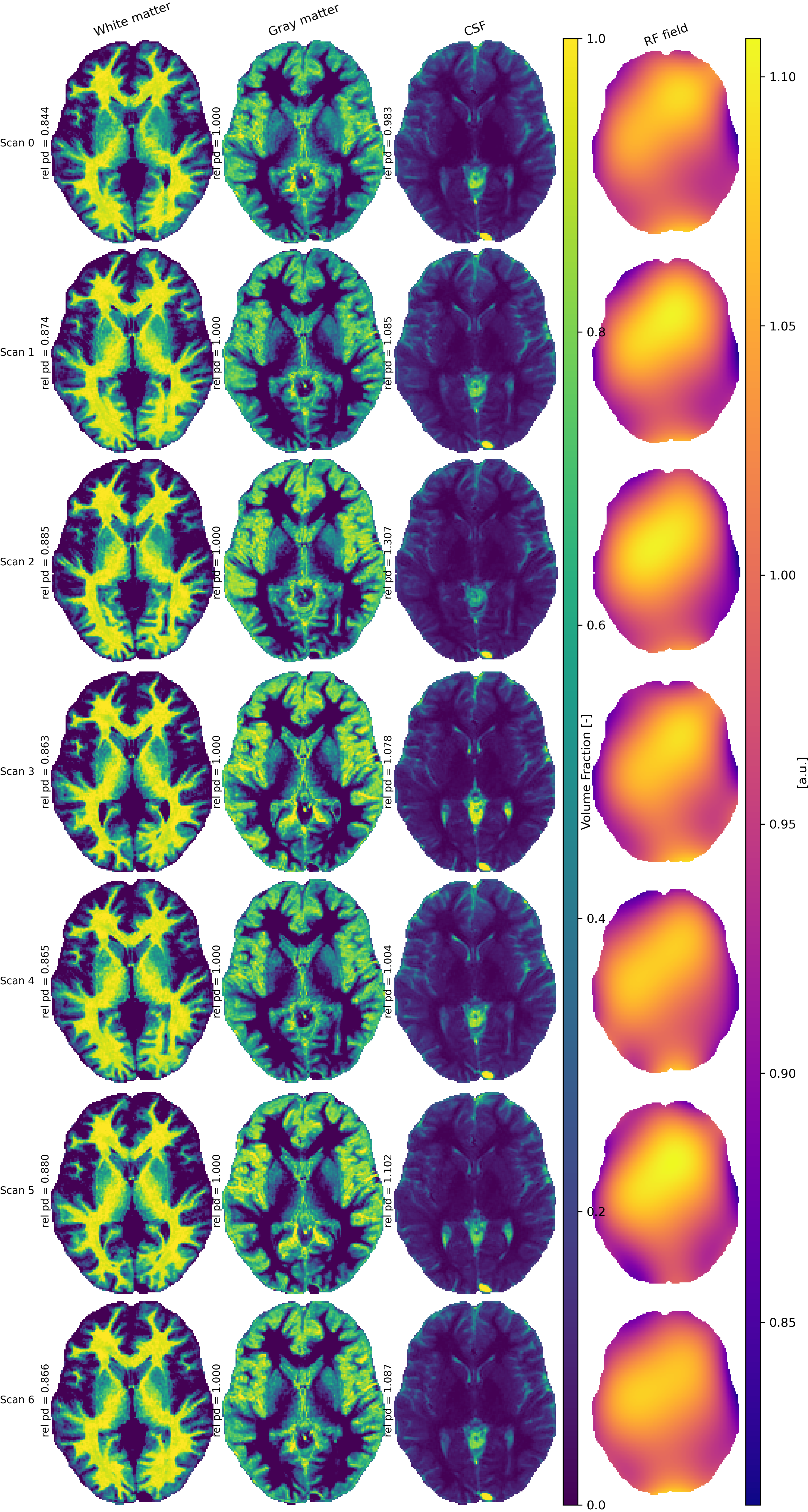
Representative volume fractions and estimated $$$B_1^-$$$-field for one subject are shown(Fig.4), results for full brain data in Fig.5.
Discussion
The proposed model effectively assumes a constant relation between the PD and magnetization for each tissue type corrected for coil sensitivities. Since tissue types are clustered based on relaxation times this seems a valid assumption, since changes in tissue pathology (including PD) will most likely result in a different $$$T_1$$$,$$$T_2$$$ component.The simulations demonstrate that tissue segmentations from MC-MRF and $$$T_1$$$w-scans may result in quite similar total tissue volume estimates, but MC-MRF outperforms the $$$T_1$$$w-approaches in regions with large partial volume effects (especially in CSF).
Grey matter was chosen as reference tissue, instead of CSF as often done. Due to the small amount of CSF present in the processed single slice data, the PD estimation for WM and GM showed to be more stable than for CSF.
Our method showed highly reproducible estimations for the single slice data and in the two full-brain datasets. The observed larger variation in CSF PD-values could be caused by the small amount of CSF in the single slice data. Analysis of more full-brain datasets will make it possible to better assess and quantify the repeatability of obtained total volumes and local partial volume estimations.
Conclusion
The proposed PD estimations make it possible to estimate quantitative tissue volume fractions from MRF data. Hence, with the proposed method it becomes possible to obtain clinically relevant accurate tissue volume measurements from MRF acquisitions enhancing robustness to partial volume effects compared to $$$T_1$$$w or single-component MRF based methods.Acknowledgements
This research (M.A. Nagtegaal) was partly funded by the Medical Delta consortium, a collaboration between the Delft University of Technology, Leiden University, Erasmus University Rotterdam, Leiden University Medical Center and Erasmus Medical Centre.
Data was acquired in the context of GE Healthcare grant (WS B-GEHC-05).
References
[1] L. Pini et al., “Brain atrophy in Alzheimer’s Disease and aging,” Ageing Research Reviews, vol. 30, pp. 25–48, Sep. 2016, doi: 10.1016/j.arr.2016.01.002.
[2] R. Heinen, W. H. Bouvy, A. M. Mendrik, M. A. Viergever, G. J. Biessels, and J. de Bresser, “Robustness of Automated Methods for Brain Volume Measurements across Different MRI Field Strengths,” PLoS ONE, vol. 11, no. 10, p. e0165719, 2016, doi: 10.1371/journal.pone.0165719.
[3] J. Tohka, “Partial volume effect modeling for segmentation and tissue classification of brain magnetic resonance images: A review,” World J Radiol, vol. 6, no. 11, pp. 855–864, Nov. 2014, doi: 10.4329/wjr.v6.i11.855.
[4] Y. Jiang, D. Ma, N. Seiberlich, V. Gulani, and M. A. Griswold, “MR fingerprinting using fast imaging with steady state precession (FISP) with spiral readout,” Magnetic Resonance in Medicine, vol. 74, no. 6, pp. 1621–1631, 2015, doi: 10.1002/mrm.25559.
[5] M. E. Poorman et al., “Magnetic resonance fingerprinting Part 1: Potential uses, current challenges, and recommendations,” Journal of Magnetic Resonance Imaging, vol. 0, no. 0, doi: 10.1002/jmri.26836.
[6] G. Buonincontri et al., “Multi-site repeatability and reproducibility of MR fingerprinting of the healthy brain at 1.5 and 3.0 T,” NeuroImage, vol. 195, pp. 362–372, Jul. 2019, doi: 10.1016/j.neuroimage.2019.03.047.
[7] G. Körzdörfer et al., “Reproducibility and Repeatability of MR Fingerprinting Relaxometry in the Human Brain,” Radiology, p. 182360, Jun. 2019, doi: 10.1148/radiol.2019182360.
[8] M. Nagtegaal, P. Koken, T. Amthor, and M. Doneva, “Fast multi-component analysis using a joint sparsity constraint for MR fingerprinting,” Magnetic Resonance in Medicine, vol. 83, no. 2, pp. 521–534, 2020, doi: 10.1002/mrm.27947.
[9] S. Volz, U. Nöth, A. Jurcoane, U. Ziemann, E. Hattingen, and R. Deichmann, “Quantitative proton density mapping: correcting the receiver sensitivity bias via pseudo proton densities,” NeuroImage, vol. 63, no. 1, pp. 540–552, Oct. 2012, doi: 10.1016/j.neuroimage.2012.06.076.
[10] B. Aubert-Broche, M. Griffin, G. B. Pike, A. C. Evans, and D. L. Collins, “Twenty New Digital Brain Phantoms for Creation of Validation Image Data Bases,” IEEE Transactions on Medical Imaging, vol. 25, no. 11, pp. 1410–1416, Nov. 2006, doi: 10.1109/TMI.2006.883453.
[11] S. M. Smith et al., “Accurate, Robust, and Automated Longitudinal and Cross-Sectional Brain Change Analysis,” NeuroImage, vol. 17, no. 1, pp. 479–489, Sep. 2002, doi: 10.1006/nimg.2002.1040. [12] C. Gaser and R. Dahnke, “CAT-a computational anatomy toolbox for the analysis of structural MRI data.”
[13] W. R. Crum, O. Camara, and D. L. G. Hill, “Generalized Overlap Measures for Evaluation and Validation in Medical Image Analysis,” IEEE Transactions on Medical Imaging, vol. 25, no. 11, pp. 1451–1461, Nov. 2006, doi: 10.1109/TMI.2006.880587.
[14] Z. Abbas, V. Gras, K. Möllenhoff, F. Keil, A.-M. Oros‐Peusquens, and N. J. Shah, “Analysis of proton‐density bias corrections based on $$$T_1$$$ measurement for robust quantification of water content in the brain at 3 Tesla,” Magnetic Resonance in Medicine, vol. 72, no. 6, pp. 1735–1745, Dec. 2014, doi: 10.1002/mrm.25086.
[15] J. Z. Bojorquez, S. Bricq, C. Acquitter, F. Brunotte, P. M. Walker, and A. Lalande, “What are normal relaxation times of tissues at 3 T?,” Magnetic Resonance Imaging, vol. 35, pp. 69–80, Jan. 2017, doi: 10.1016/j.mri.2016.08.021.
Figures