Introduction

Chemical Exchange Saturation Transfer(CEST) detects dilute solute in-vivo via water signal through the exchange of saturated proton from the solute. CEST has been used to grade glioma¹, lateralize epileptic foci² and predict proteoglycan level³. However, the CEST values itself depend on the B₁ strength. The influence of B₁ has been corrected mostly at 7T but not at 3T. The uncorrected CEST map may jeopardize the accuracy of diagnosis. Traditionally B₀/B₁ is corrected by performing first the B₀ correction followed by B₁ correction⁴. Thereby the exact same offsets have to be acquired per B₁ value. Here, we proposed a novel method that implements B₀ and B₁ correction anti-respectively (B0B1CAR) and apply this method for amide proton transfer weighted (APTw) imaging at 3T. The proposed method has higher flexibility in data sampling at different B₁ and RF offsets. Our results demonstrate that compared with the conventional method (B₀ only correction) and the B₀/B₁ correction with minimal sampled data, the proposed method halved the upper brain region's error with the cost of little increase of scan time.

Methods

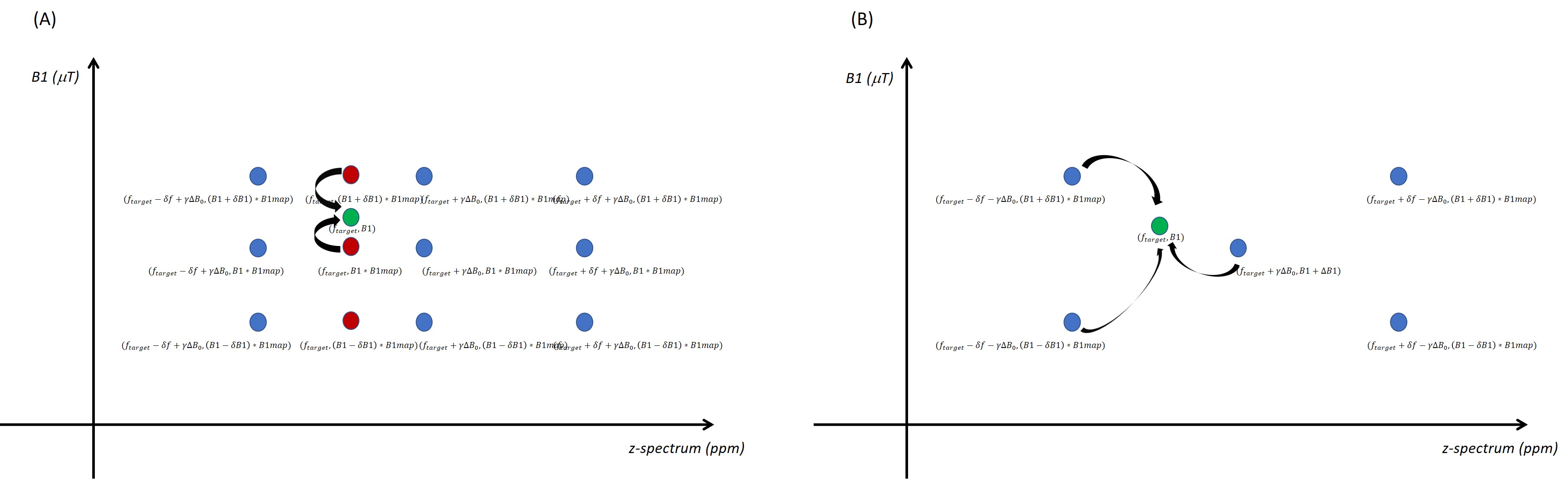
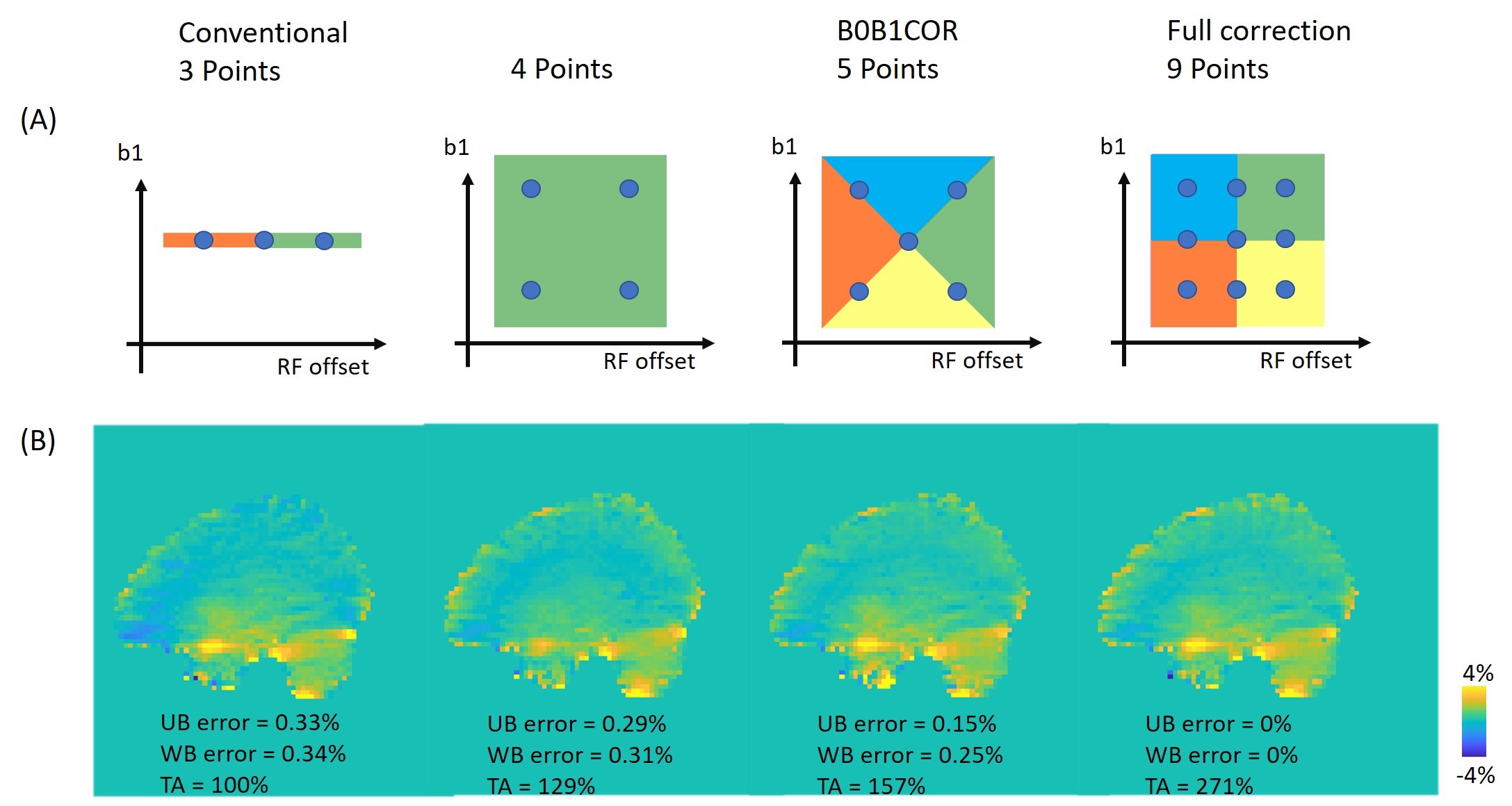
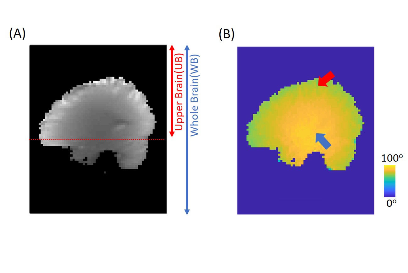
Figure 1A illustrates the conventional B₀/B₁ correction method. Step 1, the data at the target frequency offset (red dots) were interpolated for each sampled B₁ value separately. Step 2, the data at the target frequency offset and target B₁ (green dot) was interpolated by the B₀ corrected data from step 1. Figure 1B illustrates the B0B1CAR method for simultaneous B₀ and B₁ correction. The target frequency offset and B₁ data were interpolated directly by sampled data at different frequency offsets and B₁. This method has no restriction on data sampling patterns at RF offsets and B₁ values. We used SPACE to collect CEST data⁵ (TR = 3000ms, TE = 3.6ms, ETL = 165, Averages = 1.4, GRAPPA = 2 X 2, resolution = 2.75 mm³, 10 X 90ms Gaussian pulses, 10ms gap). B₁ map was collected by a pre-saturated tfl method. Multi-echo GRE with the same FOV and resolution was used to generate a field map. After correction, the data at frequency offset = ±3.5ppm, and B1 = 2μT were used to calculate APTw images by MTR asymmetry⁶. A volunteer was scanned on a 3T MR scanner (MAGNETOM Prisma, Siemens Healthcare, Erlangen, Germany). Figure 2A illustrates the data sampling and correction method in this study. Blue dots represent the sampled data at different RF offsets and B₁, and regions with different colors were interpolated from different sets of points. The conventional method is a B₀ only corrected method that is widely used⁶. For correcting B₁, a 9 points method was used with RF offsets = -300, ±3, ±3.5, ±4 ppm and a nominal B₁ of 1.6, 2, 2.4 μT. The acquired data for the other methods can be derived from Figure 2A. Mean errors were calculated for the upper brain region (UB, Figure 3A) and the whole brain region (WB) as the mean absolute difference between each method and the full correction method. The acquisition time (TA) was compared with the conventional method, which has a 100% acquisition time.

Results

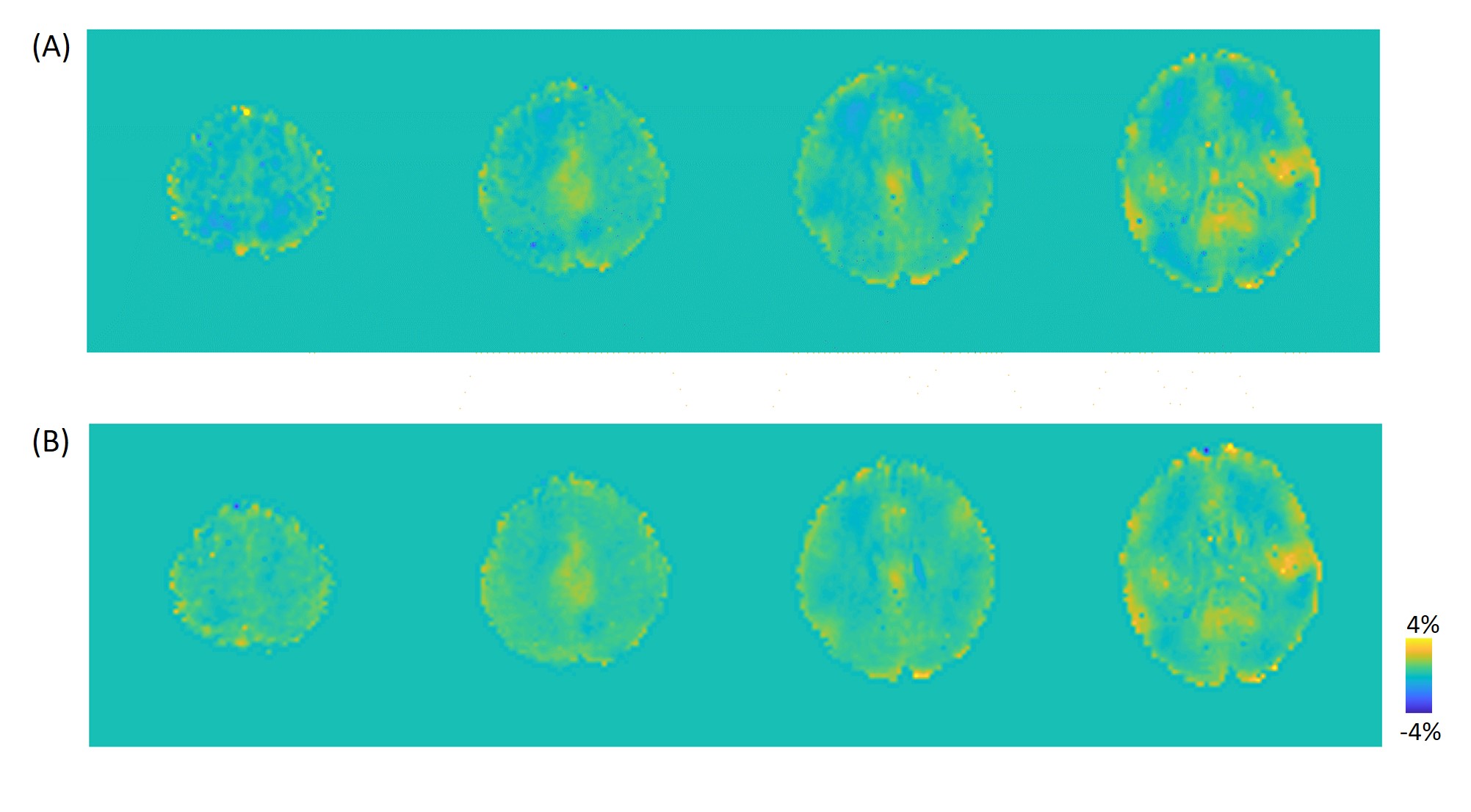
Figure 3B shows the measured flip angle map for nominal 90° flip angle. The peripheral brain region is about 70°(red arrow), and the central region is close to 90°(blue arrow). Figure 2B shows the APTw images with B₀/B₁ correction by methods illustrated in Figure 2A. The conventional 3 points method has the largest mean errors. The 4 points method, which used the minimum points required for B₀/B₁ correction, has smaller errors at the cost of 129% scan time. The B0B1CAR method has less than 50% error (0.33% -> 0.15%) in the upper brain region compared with the conventional method but less improvement for the whole brain region. The full correction method was used as a reference to quantify the goodness of correction. It used a 271% acquisition time compared with the conventional method. Figure 4 shows the sagittal view of APTw images corrected by the conventional method and B0B1CAR. The peripheral brain region of conventional APTw images shows a lower value due to a lower B₁ value.

Discussion

The conventional 3 points method was not correct for the B₁ inhomogeneity and the low B₁ value caused a higher error in APTw images near the peripheral brain region. The 4 points method used the minimal sampled data for both B₀ and B₁ correction, but the error only reduced marginally compared with the conventional method. Compared with the 4 points method, B0B1CAR acquired one more data point for B0/B1 correction, and the upper brain's error almost halved. However, the error in the whole brain region was only reduced by 0.06%. We hypothesize that the B0B1CAR with only 5 points was not enough for the region with high off-resonance.

Conclusion

The proposed B0B1CAR method provides a more flexible data sampling method for simultaneous B₀ and B₁ correction in CEST imaging. We demonstrate that B0B1CAR with 5 points can correct for B₀ and B₁ artifact efficiently in the upper brain region with almost halved error, and only one more data is required on each side of the z spectrum than the 4 points method.

Acknowledgements

No acknowledgement found.