1481
Accelerated Fitting for Quantitative Magnetization Transfer in Glioblastoma Multiforme Patients with Uncertainty using Deep Learning1Medical Biophysics, University of Toronto, Toronto, ON, Canada, 2Department of Physical Sciences, Sunnybrook Research Institute, Toronto, ON, Canada, 3Department of Radiation Oncology, Sunnybrook Health Sciences Centre, Toronto, ON, Canada, 4Department of Radiation Oncology, University of Toronto, Toronto, ON, Canada
Synopsis
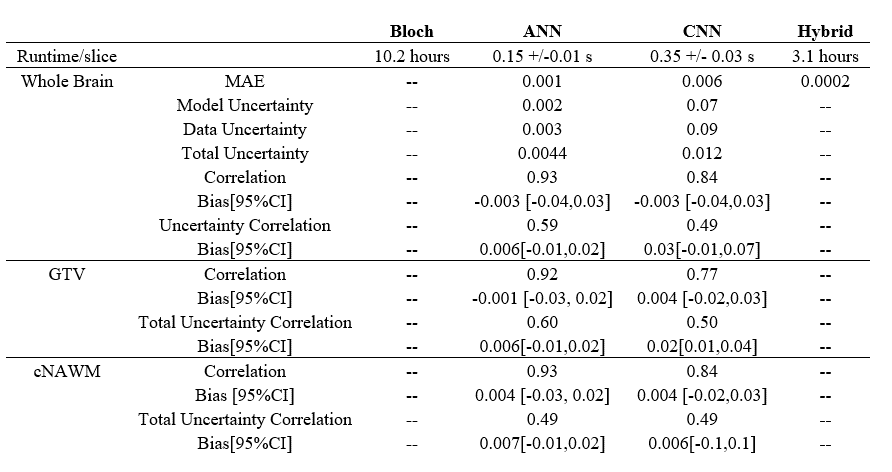
qMT has been suggested as a biomarker in Glioblastoma patients. However, reconstruction involves a computationally expensive fitting procedure involving the Bloch-McConnell equations. In this work, the use of neural networks was investigated to perform the fit and to compute uncertainty heatmaps to identify regions of potential error. The dataset consisted of 164 scans from N=41 glioblastoma patients (33=training, 8=testing). Models were evaluated using MAE and correlation in the whole-head volumes and specific ROIs. The model output agreed with a conventional curve-fitting algorithm (r=0.93, and <1% error) with speed up factors of 240000x. Uncertainty predictions were correlated with prediction error (r=0.59).
Introduction
Quantitative magnetization transfer1 (qMT) is a potential biomarker for monitoring glioblastoma (GBM) response to chemo-radiation therapy, without the need for contrast administration2,3. A major limitation of qMT is the long fitting time required to obtain parametric maps. Fast model fitting is a prerequisite for certain applications, including daily radiotherapy adaptation based on quantitative MRI. Neural networks have been previously suggested for qMT fitting4,5 but were limited to healthy patients. Our study expands on previous works by including GBM patients and computes the uncertainty on network predictions. We also investigated the use of the network outputs as initialization for a conventional reconstruction procedure, non-linear least-squares fit of the Bloch-McConnell equations6.Methods
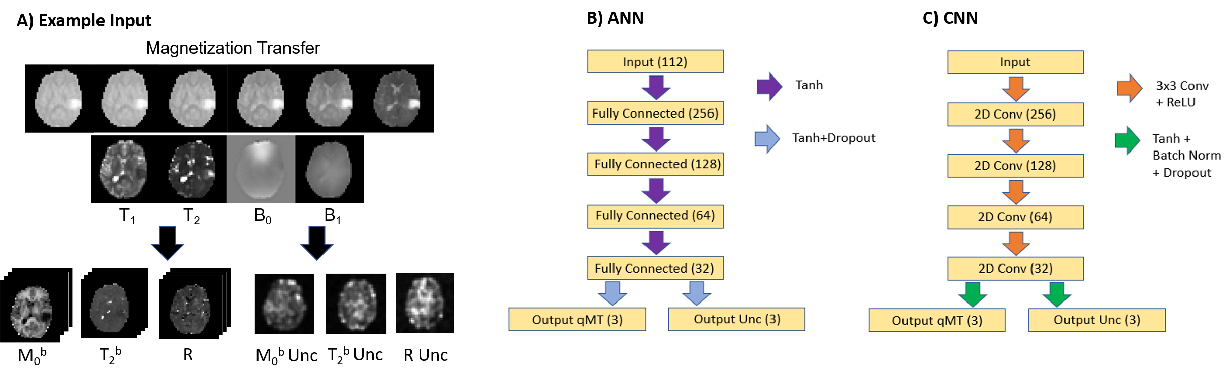
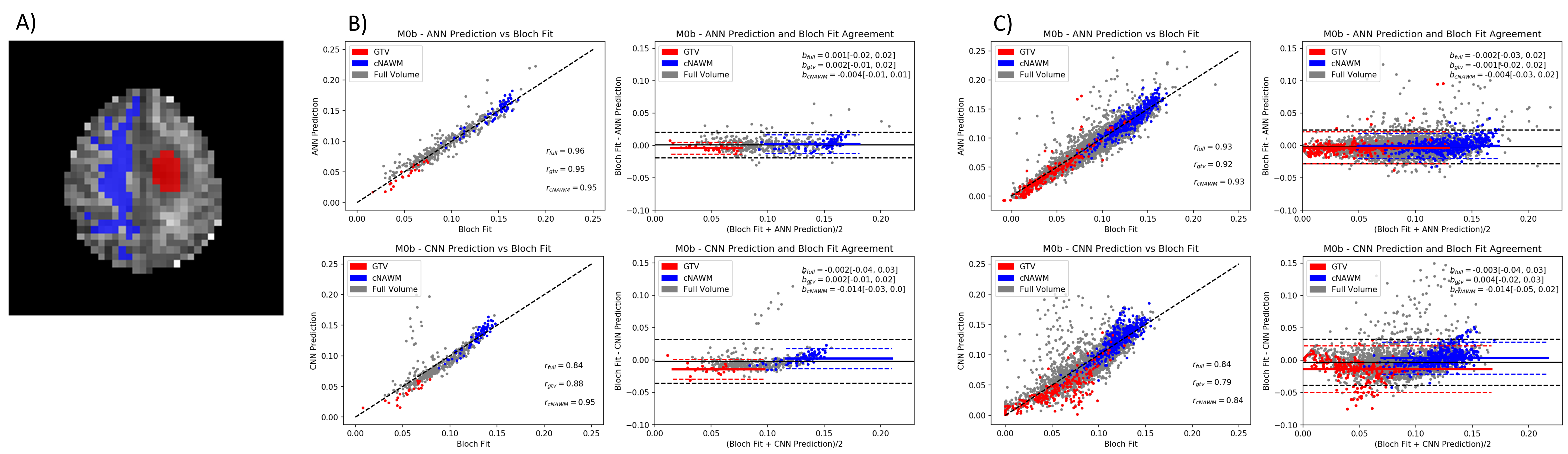
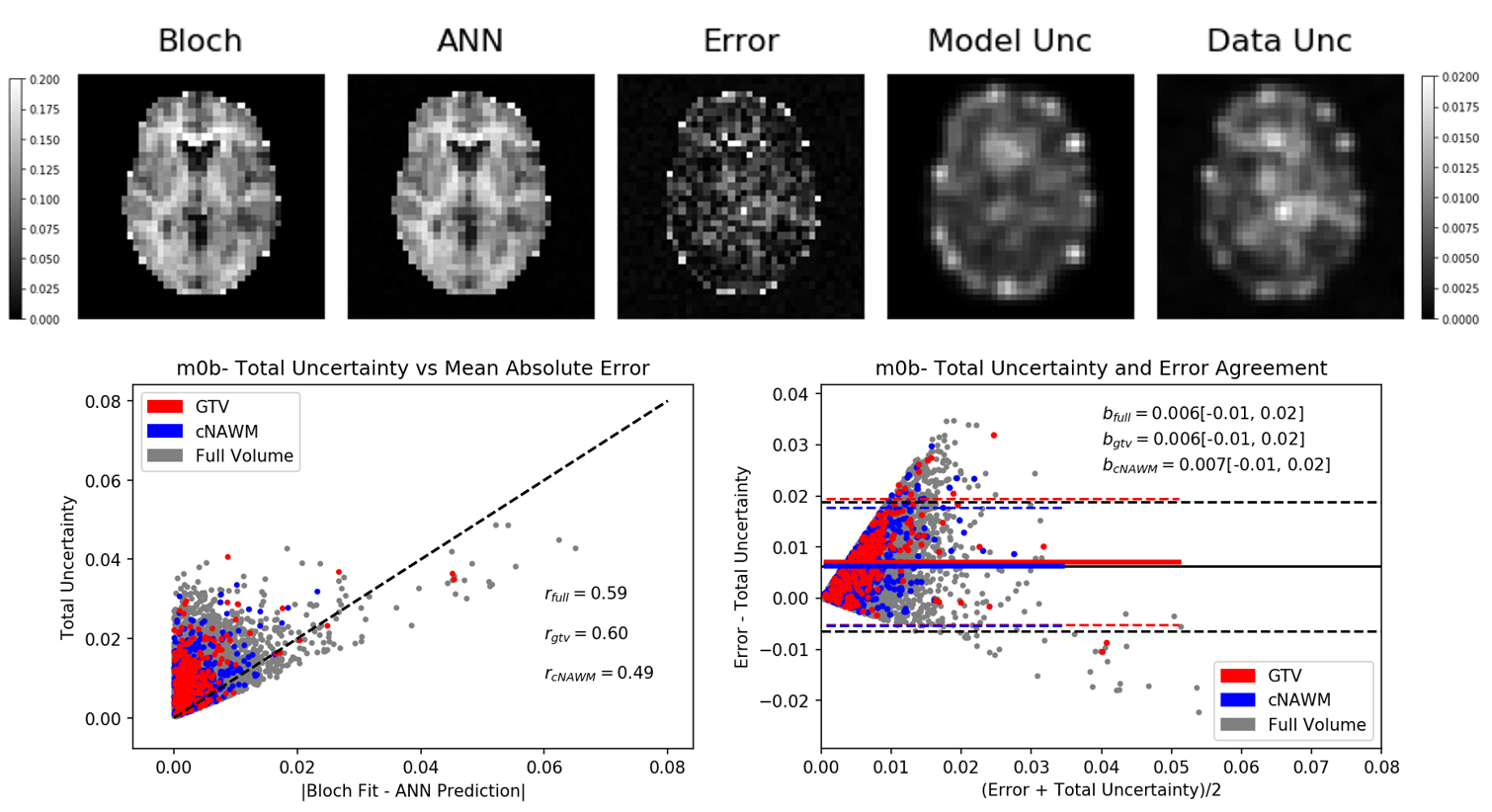
The dataset consisted 41 GBM patients (164 total scans) who underwent radiation treatment3. Scans were performed on a Philips Ingenia 1.5T. Four qMT scans were acquired from each patient: before treatment, at the 10th treatment fraction, 20th treatment fraction, and at 1-month post-chemoradiation. Patients were grouped for training (n=33) and testing (n=8). The network input was a set of T1, T2, B0, B1 maps and 18 MT saturation frequency offsets at 6 different B1 amplitude/duration. Images were downsampled to a resolution of 5.0x5.0x5.0 mm3. Input features were standardized. Padding of 1 was added when using the CNN. The outputs were the qMT parameters; the semisolid fraction (M0b), the exchange rate (R), and the T2 times for the bound pool (T2b). The output of the non-linear least-squares fit of the Bloch McConnell equations6 was used as ground truth for network training and evaluation. Model outputs were compared over the entire brain, in the gross tumor volume (GTV, taken from clinical treatment planning) and contralateral normal-appearing white matter (cNAWM, determined with FSL-FAST7). Two network architectures were investigated: an artificial neural network (ANN), and a convolutional neural network (CNN). The network architecture and implementation details are described in figure 1. Uncertainty predictions were obtained from the networks following the procedure described by Kendall8. Uncertainty over model parameters (model uncertainty) was determined using Monte Carlo dropout by taking the variance of 50 dropout samples. Uncertainty due to noise in the input data (data uncertainty) was obtained the modifying the mean squared loss function to include variance, ($$$\sigma^2$$$), $$$MSE_{unc} = (ground truth-output)^2 / \sigma^2 + ln(\sigma^2)$$$ and splitting the final layer of the networks to output a prediction of $$$\sigma^2$$$. We additionally tested using the output of the ANN to initialize the traditional Bloch-McConnell fit (denoted ‘hybrid’), rather than using arbitrary values chosen a priori. The runtime of the hybrid method was compared to the normal fitting runtime (approximately 10 hours).Results
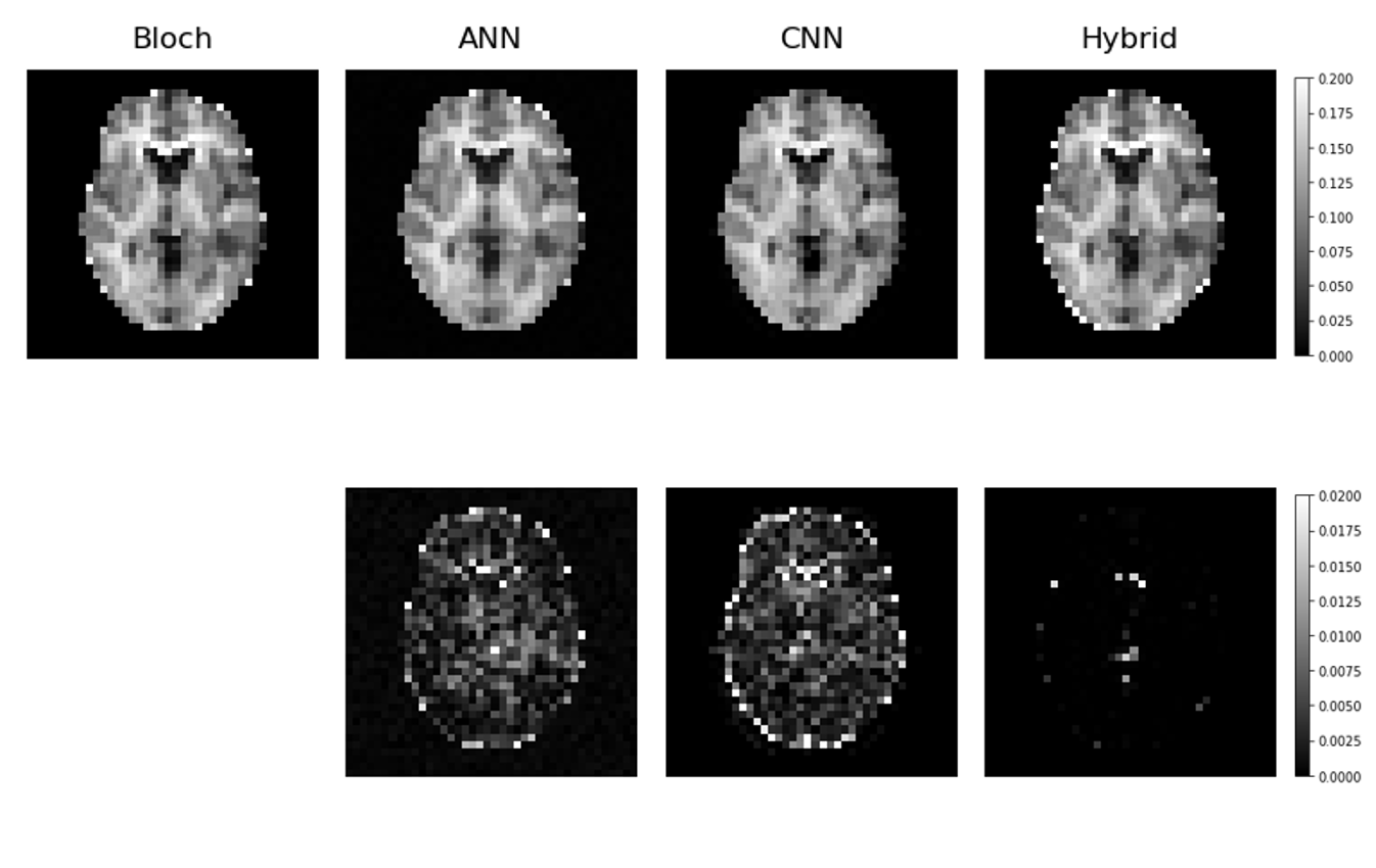
Network training took approximately 30 min for the ANN and 90 mins for the CNN. Once trained, qMT parameters with uncertainty predictions could be generated in less than one second on both architectures. Using the output of the ANN on the traditional fit reduced the average run time from approximately 10 hours per slice to slightly over 3 hours per slice. The mean absolute error (MAE) of M0b predicted by each model was, ANN=0.001, CNN=0.006, and hybrid=0.0002 Fig. 2 shows an example output of semisolid fraction for each method and the difference maps compared to the ground truth. Fig. 3 shows the correlation and bias of M0b between the ground truth and ANN output of a slice over the GTV, cNAWM, and the full brain volume using Bland-Altman analysis. Fig. 4 similarly shows the correlation and bias of ANN uncertainty predictions the absolute error between predictions and the Bloch fit. Uncertainty was overpredicted, serving as an upper bound on error.Discussion
qMT fitting on GBM patients performed using an ANN was accurate compared to a conventional fitting method using the Bloch-McConnell equations in all three regions of interest, including the GTV. The MAE of M0b between the ANN and Bloch-McConnell fit was within the standard deviation across the patients for each region3. In this experiment, the ANN model output was more accurate than the CNN and had a higher correlation with ground truth over the eight-patient test set. Higher resolution images may improve CNN performance in future works. For both networks, the time required to generate qMT images was less than a second, compared to the 10 hours required to generate the images with least-squares fitting. The hybrid model was investigated as a more interpretable method that may be more robust at handling out of distribution input (data the model has not seen before) compared to the neural networks alone, while still reducing the runtime of the traditional workflow. This is likely to increase the clinical adoption of online reconstruction for dose adaptation. Uncertainty predictions to automatically determine potentially incorrect voxels for quality assurance is desirable for clinical implementation. Uncertainty predictions were found to be correlated with errors between the ground truth and network output. However, uncertainty was overpredicted compared to the observed error in each ROI. Future work will include uncertainty calibration to address underpredicted uncertainties.Conclusion
This study demonstrated that qMT fitting using neural networks was accurate when compared to traditional non-linear least-squares fitting. The increased efficiency and associated uncertainty predictions are expected to facilitate clinical implementation of qMT as a biomarker for GBM progression.Acknowledgements
We gratefully acknowledge funding from NSERC (RGPIN-2017-06596) and NVIDIA Corporation with the donation of the GPUs used in this work.References
1. Kucharczyk W, Macdonald P.M, Stanisz G.J, Henkelman R.M. Relaxivity and magnetization transfer of white matter lipids at MR imaging: Importance of cerebrosides and pH. Radiology. 1994;192:521–529.
2. Mehrabian H, Myrehaug S, Soliman H, Sahgal A, Stanisz GJ. Quantitative Magnetization Transfer in Monitoring Glioblastoma (GBM) Response to Therapy. Sci Rep. 2018;8(1):2475.
3. Chan R. W, Chen H, Myrehaug S, Atenafu E. G, Stanisz G. J, Stewart J, Maralani P. J, Chan A. K. M, Daghighi S, Ruschin M, Das S, Perry J, Czarnota G. J, Sahgal A, Lau A. Z. Quantitative CEST and MT at 1.5T for monitoring treatment response in glioblastoma: early and late tumor progression during chemoradiation. Journal of Neuro-Oncology. 2020;1–12.
4. Luu H. M, Kim D, Kim J, Choi S, Park S. qMTNet: Accelerated quantitative magnetization transfer imaging with artificial neural networks. Magnetic Resonance in Medicine. 2021;85(1): 298–308.
5. Kim B, Schär M, Park H. W, Heo H. Y. A deep learning approach for magnetization transfer contrast MR fingerprinting and chemical exchange saturation transfer imaging. NeuroImage. 2020; 221:117165. 6. Chan R. W, Myrehaug S, Stanisz G. J, Sahgal A, Lau A. Z. Quantification of pulsed saturation transfer at 1.5T and 3T. Magnetic Resonance in Medicine. 2019;82(5);1684–1699.
7. Zhang Y, Brady M, Smith S. Segmentation of brain MR images through a hidden Markov random field model and the expectation-maximization algorithm. IEEE Trans Med Imag. 2001;20(1):45-57.
8. Kendall A, Gal Y. What uncertainties do we need in Bayesian deep learning for computer vision? Adv. Neural Inf. Process. Syst. 30. 2017;5580–5590
9. Paszke A. et al. PyTorch: An Imperative Style, High-Performance Deep Learning Library. Adv. Neural Inf. Process Syst. 32. 2019;8024–8035.
Figures