INTRODUCTION:

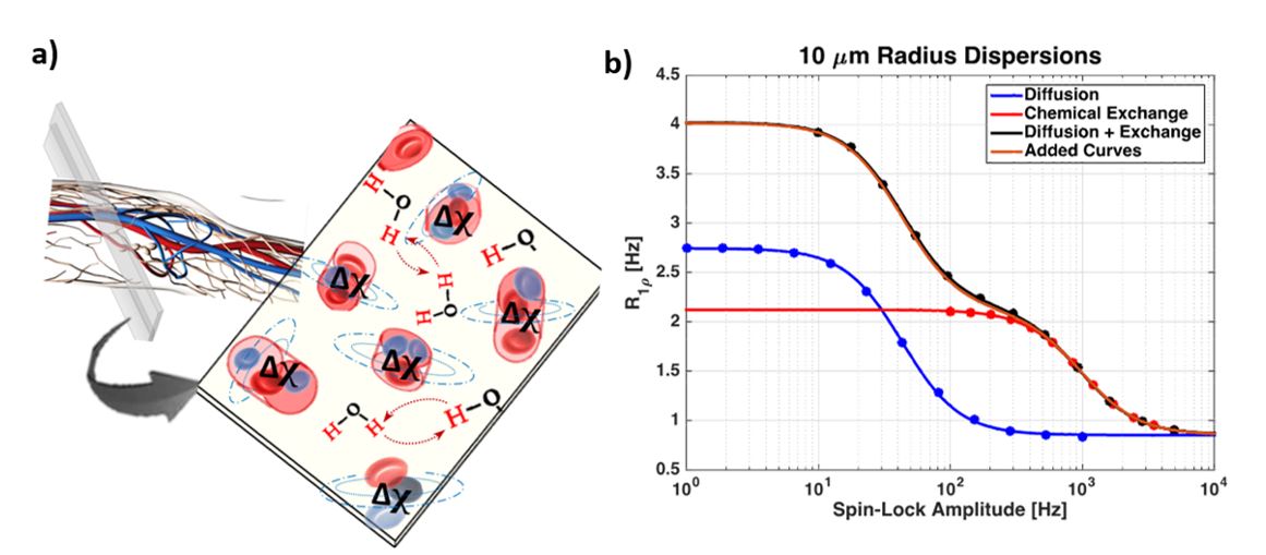
Measurements of the spin-lattice relaxation rate in the rotating frame (R_1ρ=1/T_1ρ), using spin-locking pulse sequences, are sensitive to local magnetic field fluctuations around the frequency of an applied locking pulse.¹ R_1ρ values vary as a function of the magnitude of the locking field frequency (FSL), and measurements of this variation (or dispersion) allow the derivation of intrinsic tissue properties. Recently, it has been shown that R_1ρ dispersion at high static magnetic fields is dominated by chemical exchange (R_1ρ^Ex) and diffusion (R_1ρ^Diff) effects.² Because the time scales of R_1ρ^Ex and R_1ρ^Diff are so different, these two processes are readily separated, as shown in Figure 1.³ Most in vivo studies of R_1ρ dispersion have been performed at relatively high FSL, where they emphasize the sensitivity of R_1ρ dispersion to chemical exchange.^4,5 Here we provide in-vivo results supporting the application of R_1ρ dispersion at lower FSL to quantify the signal dephasing caused by diffusion of tissue water molecules within field gradients produced by local magnetic field inhomogeneities.^3,6 We present model fit parameters from R_1ρ dispersion measurements of human skeletal muscle to estimate vascular spacing.

MATERIALS & METHODS:

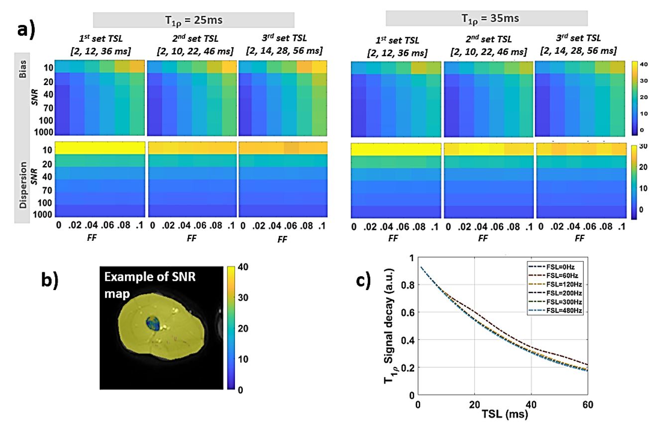
Theory of R_1ρ dispersion at low FSL: Diffusion within spatially varying magnetic field gradients induced by susceptibility variations produces a time-dependent modulation of spin frequencies that results in a net loss of transverse magnetization. These losses may be partially reduced by application of a locking field. For example, if the local field gradient varies sinusoidally with position x, it can be formulated as B₀^loc=(√2g/q)sin(qx), where g is the mean gradient strength and q is the spatial frequency of the gradient field. The contribution of this local field gradient to the relaxation rate from random diffusion is R_1ρ^Diff=γ²g²D/((q²D)²+ω₁²), where D is the self-diffusion coefficient and ω₁ is the FSL.³ In tissues, microscopic field gradients may be produced by, for example, the susceptibility differences between tissue and blood, so that q reflects the effective width of the spatial frequency spectrum of inhomogeneities corresponding to vasculature. Images acquired with different values of ω₁ can be combined to specifically portray τ_c= 1/q²D, a correlation time which is a direct measure of the sizes and spacings of the capillaries, arterioles, and venules. Variations such as those produced by small micro-vessels of dimension d correspond to values of q≈π/d.
Numerical simulation: Monte-Carlo simulations were used to assess the effect of noise and residual unsuppressed fat signal on the bias and dispersion of measured T_1ρ values in different conditions. The signals were generated using a monoexponential model with an additional term for the residual fat signal; f_f=exp(-bD_f). Different selections of TSL values were simulated along with the effects of added zero-mean Gaussian noise to vary SNR values.
MRI acquisition: 2D and 3D T_1ρ images were acquired from the lower extremity skeletal muscle in healthy young subjects, positioned supine, feet first, using a 3T Ingenia-CX MRI scanner (Philips Healthcare). Spin-lock images were acquired with a TSE readout following a 90_x-τ/2_y-180_y-τ/2_−y-90_x pulse preparation with SPIR fat suppression and PB volume shim.

RESULTS & DISCUSSION:

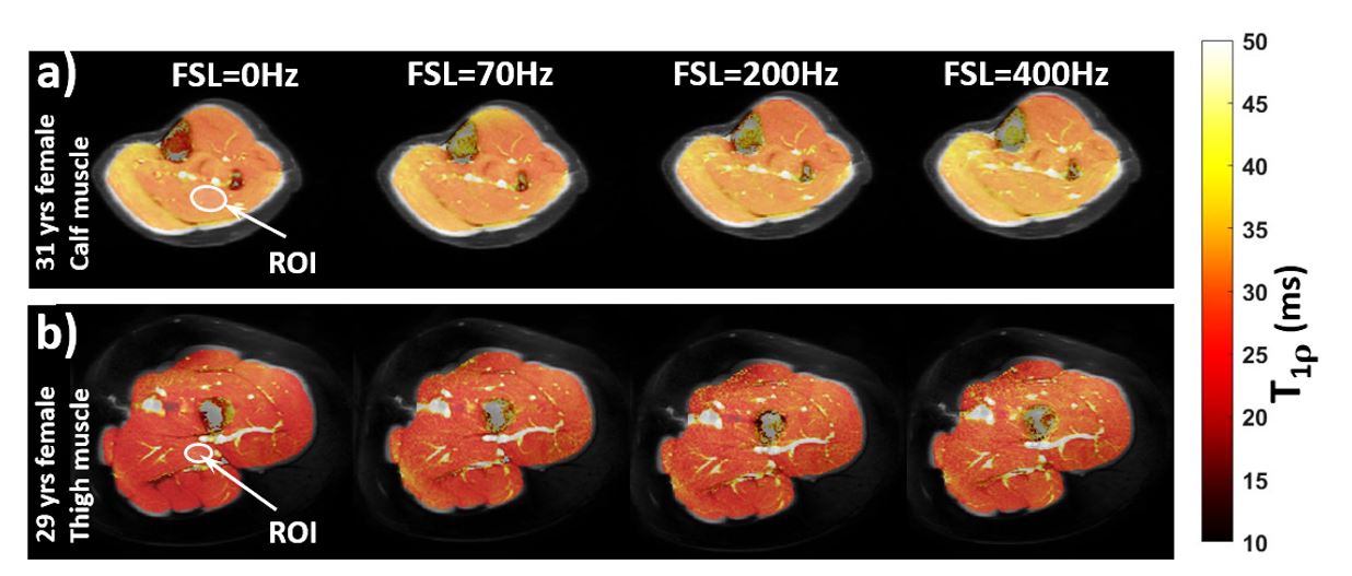
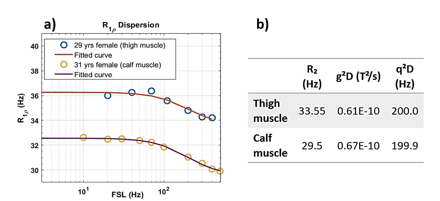
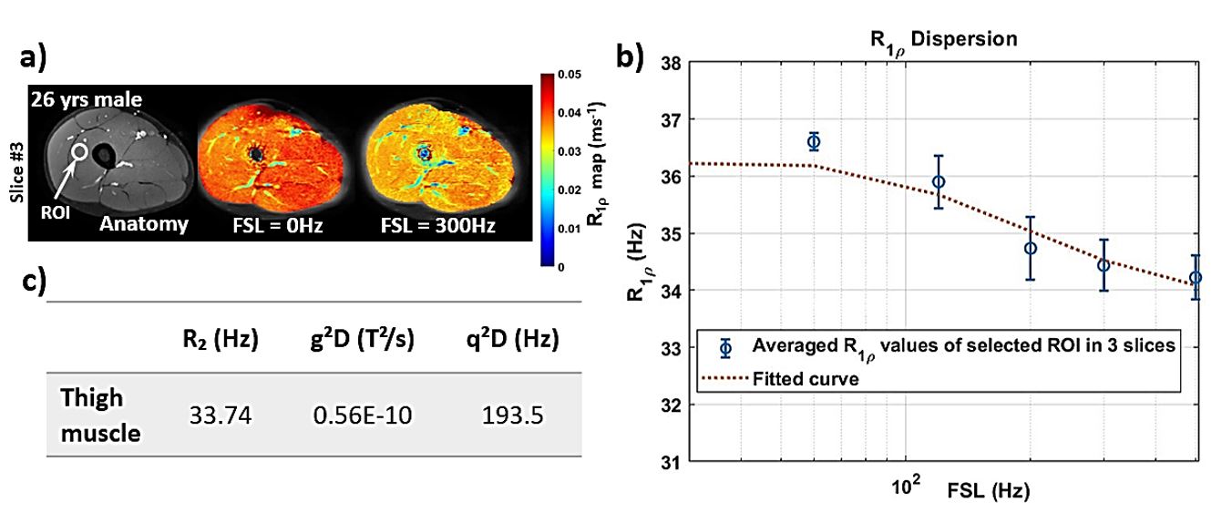
Fig.2 shows calculated T_1ρ maps of the leg. There is a slight increase in T_1ρ values at increasing spin locking fields as predicted. Fig.3 shows the quantitative R_1ρ dispersion curves and the fitted parameters from selected ROIs in calf and thigh muscles. Both dispersions reveal similar spatial frequency (q) and magnetic gradient strength (g). Moreover, if D=2x10^-5cm²/s, then the derived length scale characterizing the intrinsic gradients is d≈10μm which is close to the dimensions of microvasculature obtained from skeletal muscle in animals.⁷ The bias and dispersion of T_1ρ were determined for a range of expected tissue properties and acquisition parameters for optimized scan times (see Fig.4a). The measured SNR data depicted in Fig.4b can be matched with the simulation results to estimate the bias and dispersion of the T_1ρ value at different sets of TSL. Simulation results demonstrate that there is no substantial difference between different sets of TSL when the SNR is higher than 40. Furthermore, shorter TSL minimizes the adverse contributions of residual fat signal and B0-offset frequency. 3D-T_1ρ images were collected with the optimized series of TSL and a smaller number of FSL in 3 slices from the mid thigh. The measured R_1ρ dispersion within a clinically achievable scan time shows similar behavior to the 2D-R_1ρ dispersion measured in the thigh and calf skeletal muscles.

CONCLUSION:

R_1ρ dispersion imaging at low locking field amplitudes along with appropriate analyses may be applied to derive new types of parametric image information based on diffusion effects. The in-vivo results suggest we can use this approach to measure novel aspects of tissue microstructure including geometrical properties of the microvasculature. However, because of the complexity and contribution of both chemical exchange and diffusion effects to the R_1ρ dispersion, a definite conclusion cannot be stated, and further investigation such as ex-vivo validation studies should be performed.

Acknowledgements

No acknowledgement found.