Introduction

The design of the preparation period is crucial for a CEST experiment as the maximum saturation effect on water depends largely on the efficiency of the radiofrequency pulses during the preparation¹. Thus, the parameters defining the preparation period, such as RF pulse shape, pulse duration, and saturation duty cycle, have to be precisely defined. However, these parameters are not always provided in sufficient detail and their definition may vary in the literature². A common, easy-to-use and vendor-independent file format to share exact preparation parameters is therefore desirable. Moreover, a growing number of deep learning-based evaluation approaches for large data sets make a proper definition of input data even more important. Here, we propose the use of Pulseq³ to define CEST parameters in the open source and human-readable pulseq-file format. In addition, we implemented an interpreter sequence to apply the sequence events defined in these pulseq-files directly on an MR scanner. Finally, we provide an open source Bloch-McConnell simulation, which allows for simulation of the same pulseq-files that are played out on the scanner.

Methods

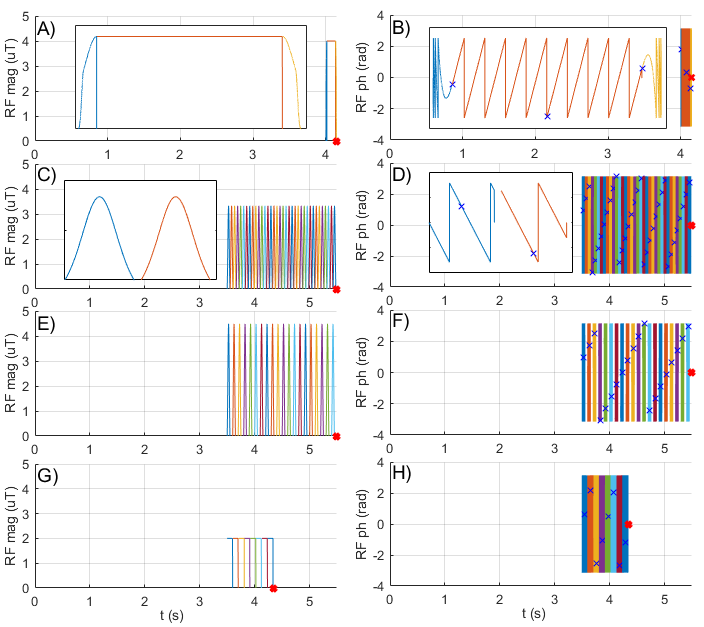
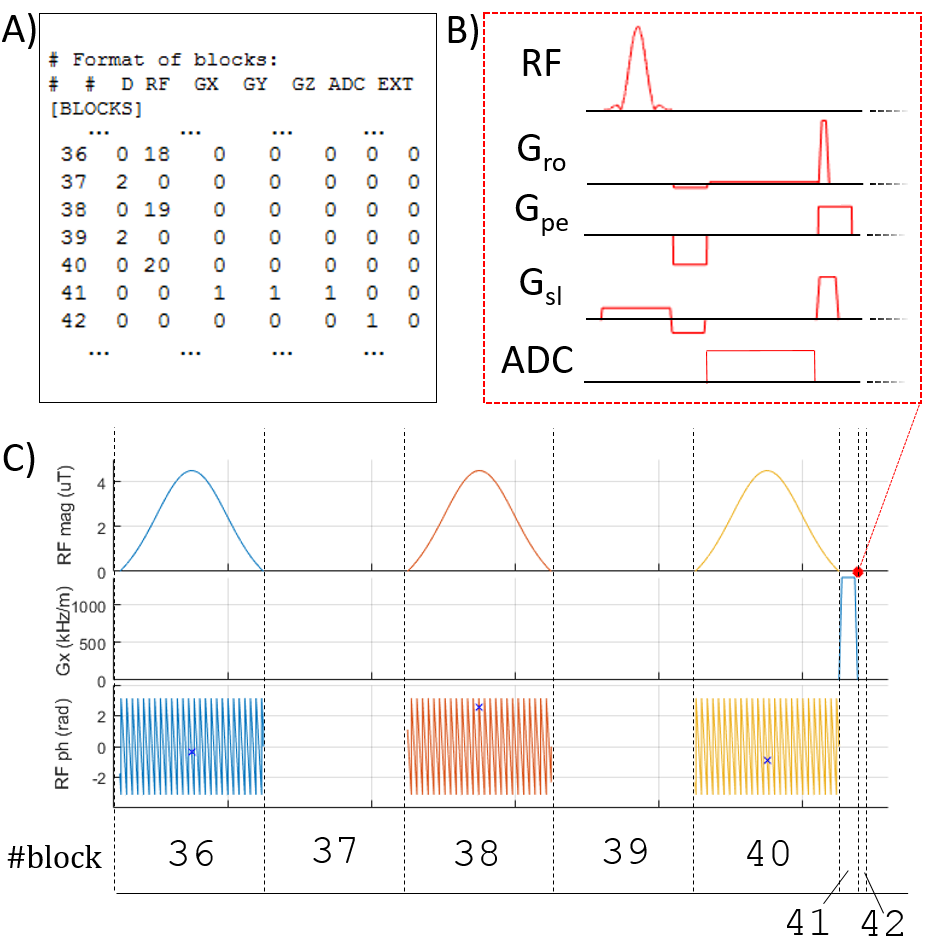
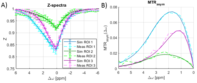
We performed two different CEST experiments in this study: (I) A phantom (L-arginine and D-glucose) Z-spectrum measurement at offsets between ±6 ppm, using an adiabatic spin-lock pulse for preparation; (II) A comparison of author-approved amide proton transfer weighted (APTw) protocols (APTw_3T_001⁴, APTw_3T_002⁵, APTw_3T_003⁶), commonly used for brain tumor studies⁷, in a healthy volunteer who provided written informed consent to the institutionally approved protocol. A sequence diagram of the RF pulses during the preparation period for these measurements is shown in Figure 1. MRI measurements were performed on a clinical 3T system (Siemens Healthineers, Germany). The original Pulseq interpreter sequence for Siemens IDEA was adapted, such that it can be used as a sequence building block (SBB), and then implemented into a 3D GRE sequence⁸. In this way, the SBB plays out the CEST preparation events defined in the pulseq-file, but the native readout sequence is used to acquire the signal (Figure 2). All CEST measurements were linearly corrected for B₀ inhomogeneity using the WASABI⁹ method. In addition, we developed an open source Bloch-McConnell simulation that loops through the pulseq-file and performs simulations of the sequence events. It was used to simulate the events defined in the pulseq-file of the phantom experiment for ROIs drawn in vials with 1) 50 mM L-arg, pH=5.55; 2) 50 mM L-arg, pH=4.01 and 3) 66 mM Glc, pH=6.52. For ROIs 1) and 2) a two-pool model¹⁰ and for ROI 3) a five-pool model¹¹ was simulated.

Results

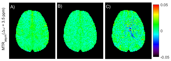
The exact definition of the saturation pulses in the pulseq-file and the multiple-pool model led to a good match between measurement and simulation (Figure 3). In vivo MTR_asym maps for the three different APTw protocols are shown in Figure 4 and despite the use of different saturation parameters, they show similar contrast. This very low contrast in healthy brain is expected, as the APTw-imaging parameters are designed to yield almost no contrast in healthy brain¹².

Discussion

Using Pulseq allows for a simple yet precise definition of CEST preparation periods in e.g. MATLAB (The Mathworks Inc., USA) or python. The pulseq-files are human-readable, allowing for a straightforward comparison. Most important, the definition of the CEST preparation period is inherently complete, facilitating total reproducibility. By adapting the source code of the Pulseq interpreter sequence to the SBB concept of the Siemens IDEA framework, we were able to use it as a sequence building block in established MR sequences and subsequently run CEST experiments on a clinical 3T scanner. Hence, we combined the full flexibility of Pulseq with sophisticated readout methods of native sequences to generate an easy-to-use and flexible method for reproducible CEST measurements. In a different study using this method¹³, we were able to apply the same CEST preparation periods on Siemens scanners built upon different hardware components and running different software versions. Furthermore, it is generally possible to transfer the approach to GE and Bruker systems where Pulseq implementations have been demonstrated³, potentially enabling coherent multi-site, multi-vendor studies. Application to other vendors is similarly possible, but would require vendor-specific interpreter software to be developed.
In addition, our software provides a Bloch-McConnell simulation tool for pulseq-files to simulate the exact same CEST preparation period that is played out by the interpreter on the scanner. This eliminates possible sources of errors from transferring simulation results to the sequence source code and vice versa. Moreover, different protocols can be compared and optimized easily in simulations and at same time be directly used on the scanner.
Finally, we provide a platform, where researchers can make their protocols available (https://pulseq-cest.github.io/) in the Pulseq standard. The pulseq-files of the protocols used in this study can also be found there. We hope that with this work, we provide a valuable and needed tool for the CEST community, to exchange and test CEST preparation periods for the many different types of different CEST experiments.

Conclusion

By using the open source Pulseq sequence definition, we provide a straightforward approach to standardize, share, simulate and measure different CEST preparation schemes, which are inherently completely defined.

Acknowledgements

The authors want to thank Patrick Schuenke and Kerstin Heinecke for implementing the python version of this project.