1454

Linear projection-based CEST reconstruction – the simplest explainable AI

Felix Glang¹, Moritz Fabian², Alex German², Katrin Khakzar², Angelika Mennecke², Frederik Laun³, Burkhard Kasper⁴, Manuel Schmidt², Arnd Doerfler², Klaus Scheffler^1,5, and Moritz Zaiss^1,2
¹High-field Magnetic Resonance Center, Max Planck Institute for Biological Cybernetics, Tübingen, Germany, ²Department of Neuroradiology, University Hospital Erlangen, Erlangen, Germany, ³Institute of Radiology, University Hospital Erlangen, Erlangen, Germany, ⁴Neurology, Epilepsy Center, University Clinic of Friedrich Alexander University Erlangen-Nürnberg, Erlangen, Germany, ⁵Department of Biomedical Magnetic Resonance, Eberhard Karls University Tübingen, Tübingen, Germany

Synopsis

Evaluation of multi-parametric in vivo CEST MRI often requires complex computational processing for both field inhomogeneity correction and contrast generation. In this work, linear regression was used to obtain coefficient vectors that directly map uncorrected 7T spectra to corrected Lorentzian target parameters by simple linear projection. The method generalizes from healthy subject training data to unseen test data of both healthy subjects and tumor patients. The linear projection approach thus integrates correction of both B₀ and B₁ inhomogeneity as well as contrast generation in a single fast and interpretable computation step.

Introduction

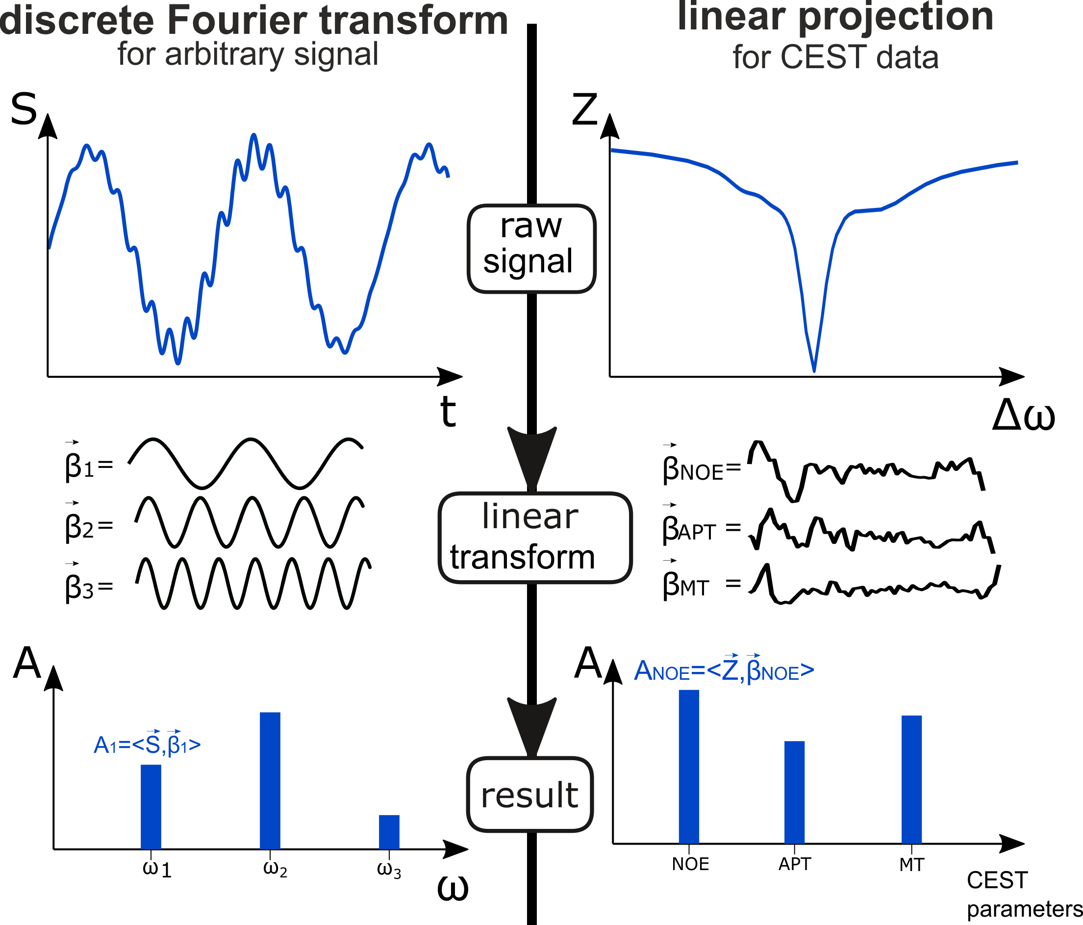
Extraction of in vivo CEST parameters often requires complex mathematical modelling for both field inhomogeneity correction and contrast generation, e.g. by non-linear curve fitting of Bloch-McConnell¹ or Lorentzian models^2–4. These are time-consuming, depend on initial and boundary conditions and thus remain difficult. Presumably, this is why simple metrics like asymmetry⁵, ratios or linear interpolations of certain points in the Z-spectra^6,7 are often preferred for CEST contrast generation. In this work, we address the question of finding the best linear combination of acquired points in the Z-spectrum to predict a desired target contrast. Such optimal linear combination weights can be found by linear regression applied to conventionally evaluated training data. Contrast generation can then be expressed analogously to a discrete Fourier transform (Figure 1, left column) as linear projection of the raw acquired data onto the respective weight vectors (Figure 1, right column).

Methods

CEST data were acquired from 6 healthy subjects and one patient with a brain tumor (glioblastoma WHO grade 4) after written informed consent at a MAGNETOM Terra 7T scanner (Siemens Healthcare GmbH, Erlangen, Germany). All in vivo examinations were approved by the local ethics committee. Homogeneous Gaussian pre-saturation (120 pulses, t_p=15 ms, t_d=10 ms) was realized using MIMOSA⁸. Image readout was a centric 3D snapshot gradient echo⁹. 56 non-equidistant frequency offsets at two saturation powers of B₁=0.72 μT and 1.00 μT were distributed between -100 and 100 ppm. A normalization image at -300 ppm was acquired after a relaxation delay of 12s.
Conventional evaluation consisted of interpolation-based B₀ and B₁ correction¹⁰, PCA denosing¹¹ and 5-pool Lorentzian fitting^2–4,12. Uncorrected but normalized Z-spectra of both B₁ levels together with respective B₁ maps from all voxels of a training dataset were assembled in an input data matrix $$$\mathbf{X}$$$ (#voxels x 110). Lorentzian parameters from each voxel and the B₀ map were likewise assembled in the target data matrix $$$\mathbf{Y}$$$ (#voxels x 17). Employing a general linear regression model, the matrix of regression coefficients $$$\hat{\mathbf{B}}$$$ for mapping $$$\mathbf{X}$$$ to $$$\mathbf{Y}$$$ was obtained by solving the ordinary least squares problem¹³ $$\hat{\mathbf{B}}=\underset{\mathbf{B}}{\text{arg min}}||\mathbf{Y}-\mathbf{XB}||_F^2=(\mathbf{X}^T \mathbf{X})^{-1}\mathbf{X}^T \mathbf{Y}$$
With that, contrasts for a new dataset can be generated as simple linear projection via matrix multiplication as $$$\mathbf{Y}_{\text{new}}=\mathbf{X}_{\text{new}}\hat{\mathbf{B}}$$$.

Results

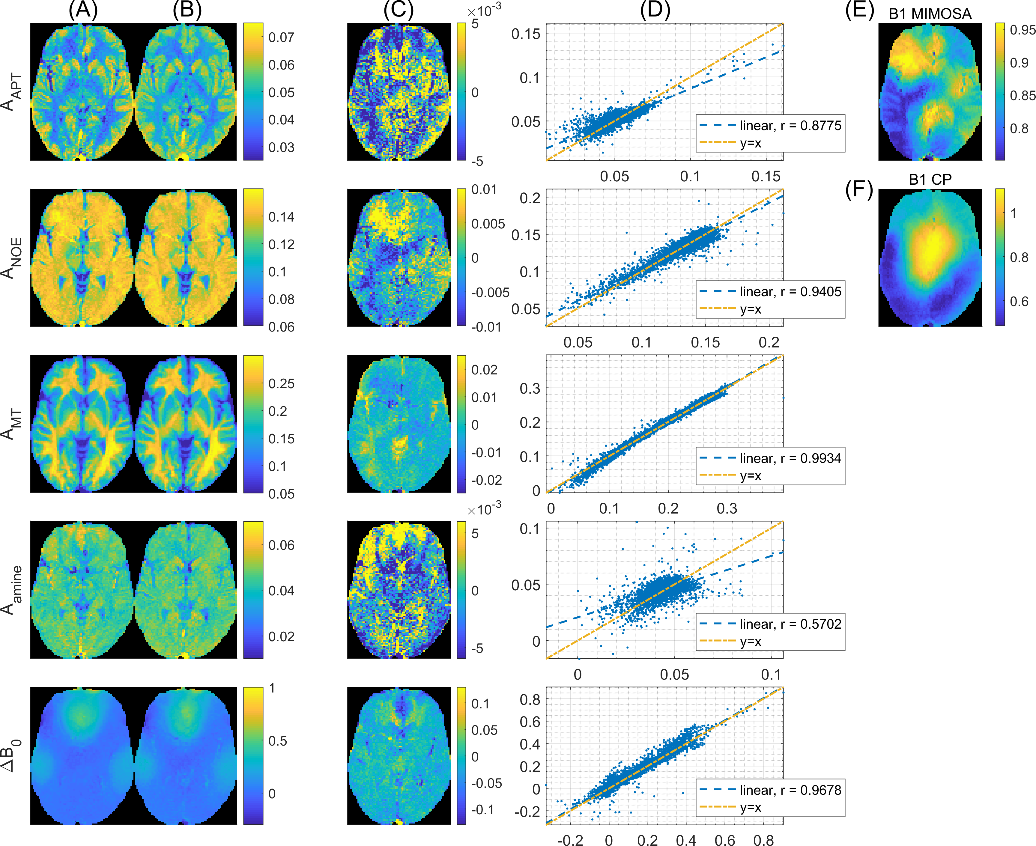
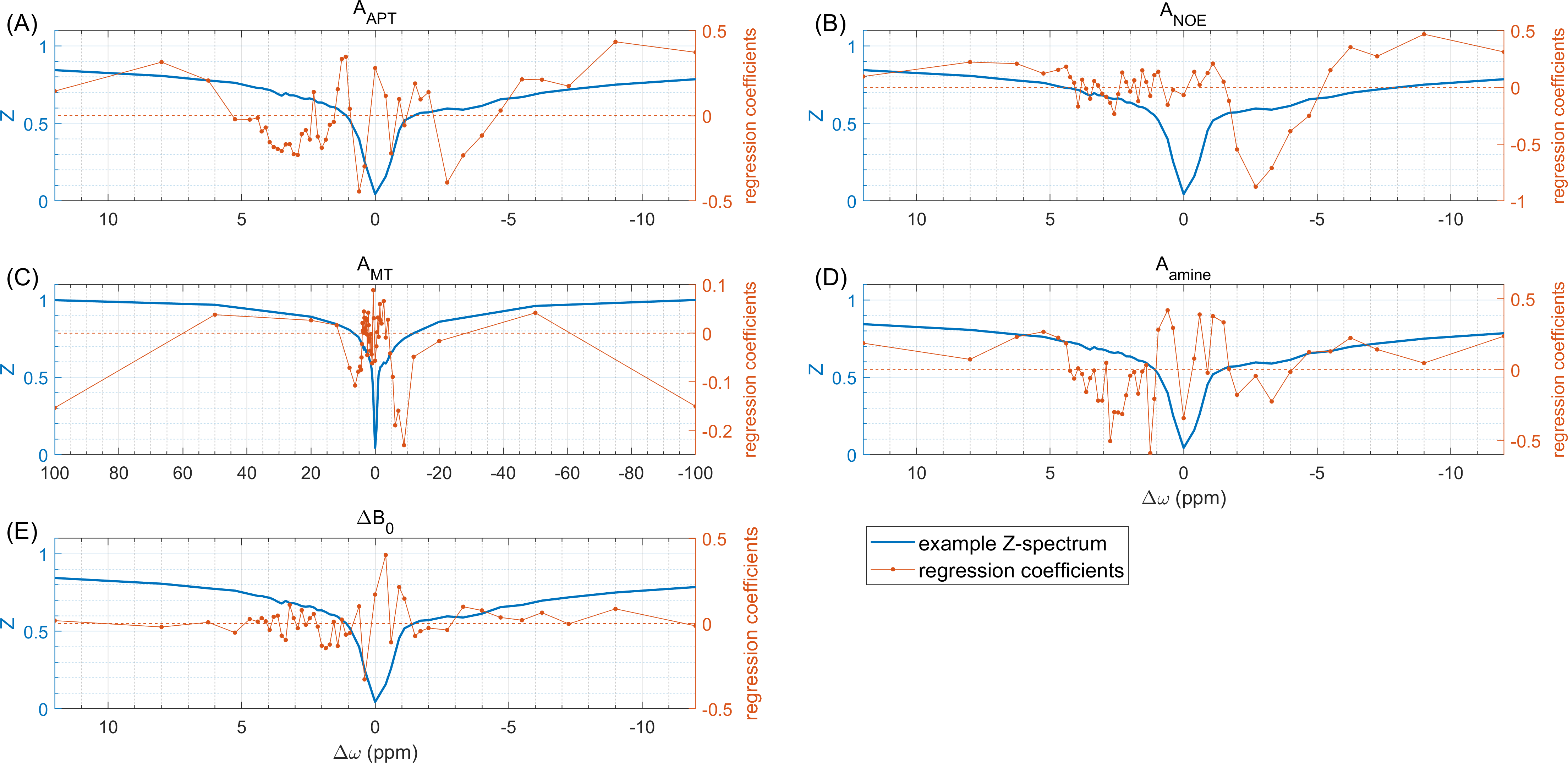
Data of 5 healthy subjects were used to obtain regression coefficients , which were then applied to a sixth healthy test dataset. The resulting maps in Figure 2 show that for APT, NOE and ssMT contrasts as well as ΔB₀, the linear projection results (Figure 2B) preserve the general contrast of the conventionally obtained ground truth maps (Figure 2A). Difference maps in Figure 2C exhibit localized deviations, which partially coincide with the MIMOSA transmit field map (Figure 2E).
In Figure 3, the obtained regression coefficients are shown. Some physically plausible patterns can be identified: For APT, there are contributions around +3.5 ppm, but also around -3.5 ppm, where NOE coefficients are highest. For amines, strongest absolute weighting occurs at 2 ppm. In case of ssMT, strongest contributions are located far off-resonant at ±100 ppm. The ΔB₀ coefficients show complex oscillatory behavior around the water peak.
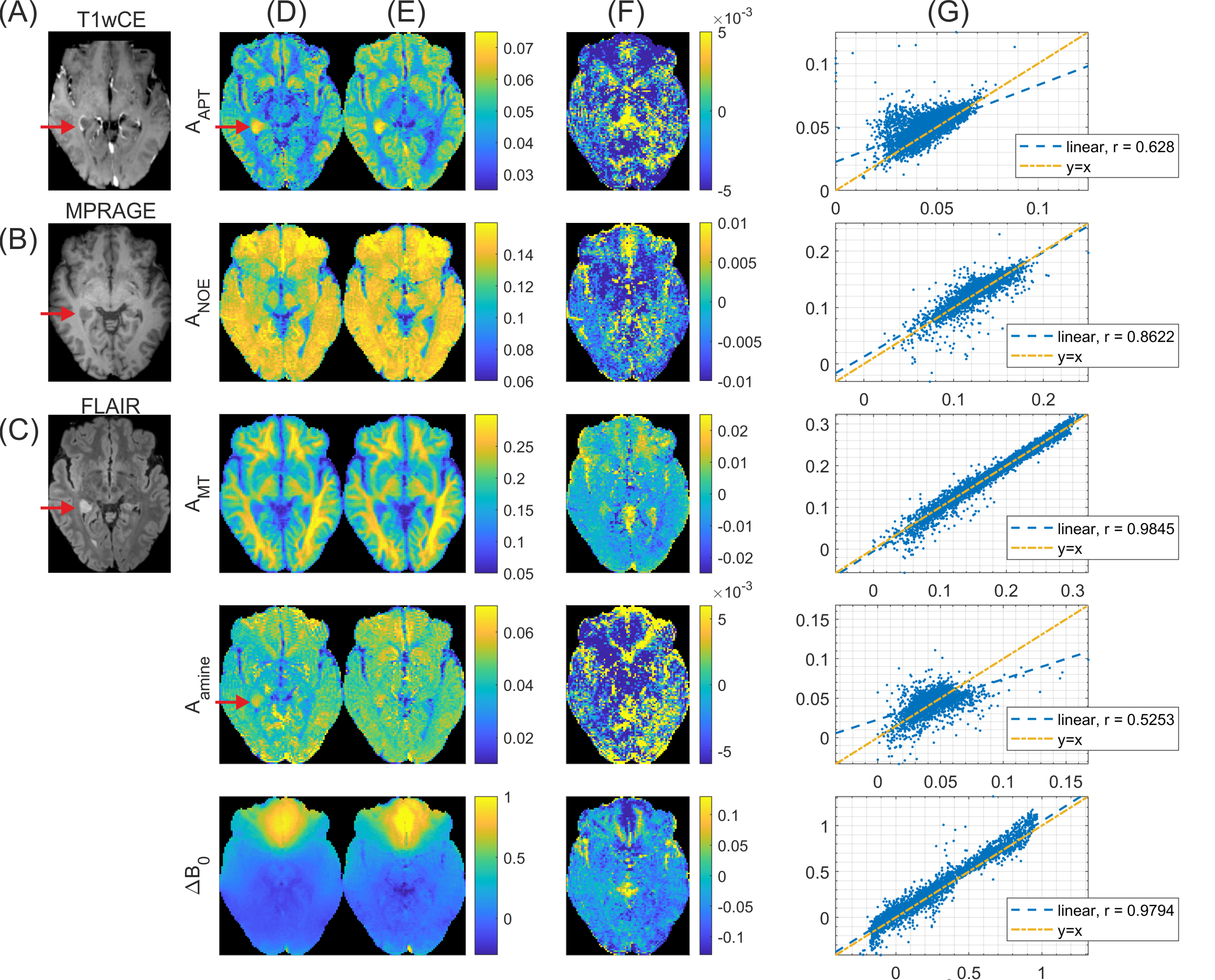
Next, generalization of the method to pathology was investigated. The same coefficients were applied to the glioblastoma patient dataset. Figure 4 shows the CEST results next to clinical contrasts for this patient. Interestingly, this tumor did not show typical gadolinium uptake (Figure 4A) as expected for glioblastoma, still amide CEST (Figure 4D, first row) showed the hyperintensity as reported previously¹⁴. Despite the regression coefficients being obtained from only healthy subject data, the linear projection approach generalizes to tumor data and the resulting maps (Figure 4E) still match the general contrast of the ground truth Lorentzian fit maps (Figure 4A), although with lower correlation coefficients (Figure 4G) than in the healthy test case (Figure 2D). Particularly, the linear projections preserve the amide hyperintensity in the tumor. Similar observations could be made when applying the linear projection approach to data from a clinical 3T scanner (results not shown).

Discussion

The linear projection approach integrates B₀ correction, B₁ correction and contrast generation into a single computation step. Both generating and applying the coefficient vectors is fast (fraction of a second) compared to conventional evaluation (several minutes) or training of neural networks (several hours). In the context of current exploration of neural networks for similar tasks^15–18, the linear transform forms the simplest learning-based approach and by its linearity allows for direct interpretation (Figure 3) and thus also guidance for more sophisticated approaches. The proposed approach can thus be considered as the simplest possible form of ‘explainable AI’¹⁹ applied to CEST MRI. The linear projection approach can be extended by L1-regularization based input feature selection (‘CEST-Lasso’), which offers the potential to accelerate CEST acquisition times significantly²⁰.

Conclusion

Multi-parametric CEST contrasts including field inhomogeneity correction can be well approximated by a simple linear projection of the acquired uncorrected Z-spectra onto regression coefficients fitted from conventionally evaluated data. The method translates from healthy to tumor patient datasets and is fast and interpretable - the latter being in contrast to neural networks employed for similar purposes. The proposed approach forms the simplest possible form of ‘explainable AI’.

Acknowledgements

Financial support of the Max-Planck Society and ERC Advanced Grant "SpreadMRI", No 834940 is gratefully acknowledged.

References

1. Liu D, Zhou J, Xue R, Zuo Z, An J, Wang DJJ. Quantitative characterization of nuclear overhauser enhancement and amide proton transfer effects in the human brain at 7 Tesla. Magnetic Resonance in Medicine 2013;70:1070–108.

2. Zaiss M, Windschuh J, Paech D, et al. Relaxation-compensated CEST-MRI of the human brain at 7T: Unbiased insight into NOE and amide signal changes in human glioblastoma. NeuroImage 2015;112:180–188.

3. Goerke S, Soehngen Y, Deshmane A, et al. Relaxation-compensated APT and rNOE CEST-MRI of human brain tumors at 3 T. Magnetic Resonance in Medicine 2019;82(2):622-632.

4. Deshmane A, Zaiss M, Lindig T, et al. 3D gradient echo snapshot CEST MRI with low power saturation for human studies at 3T. Magnetic Resonance in Medicine 2019;81:2412–2423.

5. Guivel-Scharen V, Sinnwell T, Wolff SD, Balaban RS. Detection of Proton Chemical Exchange between Metabolites and Water in Biological Tissues. Journal of Magnetic Resonance 1998;133:36–45.

6. Xu J, Zaiss M, Zu Z, et al. On the origins of chemical exchange saturation transfer (CEST) contrast in tumors at 9.4 T. NMR in Biomedicine 2014;27:406–416.

7. Jin T, Wang P, Zong X, Kim S-G. MR imaging of the amide-proton transfer effect and the pH-insensitive nuclear overhauser effect at 9.4 T. Magnetic Resonance in Medicine 2013;69:760–770.

8. Liebert A, Zaiss M, Gumbrecht R, et al. Multiple interleaved mode saturation (MIMOSA) for B1+ inhomogeneity mitigation in chemical exchange saturation transfer. Magnetic Resonance in Medicine 2019;82:693–705.

9. Zaiss M, Ehses P, Scheffler K. Snapshot-CEST: Optimizing spiral-centric-reordered gradient echo acquisition for fast and robust 3D CEST MRI at 9.4 T. NMR in Biomedicine 2018;31:e3879.

10. Windschuh J, Zaiss M, Meissner J-E, et al. Correction of B1-inhomogeneities for relaxation-compensated CEST imaging at 7 T. NMR in Biomedicine 2015;28:529–537.

11. Breitling J, Deshmane A, Goerke S, et al. Adaptive denoising for chemical exchange saturation transfer MR imaging. NMR in Biomedicine 2019;0:e4133.

12. Khakzar K. 7 tricks for 7T CEST – improving reproducibility of multi-pool evaluation. 8th International Workshop on Chemical Exchange Saturation Transfer Imaging; 2020.

13. Rencher AC, Schaalje GB. Linear models in statistics. 2nd ed. Hoboken, N.J: Wiley-Interscience; 2008.

14. Paech D, Dreher C, Regnery S, et al. Relaxation-compensated amide proton transfer (APT) MRI signal intensity is associated with survival and progression in high-grade glioma patients. Eur Radiol 2019;29:4957–4967.

15. Zaiss M, Deshmane A, Schuppert M, et al. DeepCEST: 9.4 T Chemical exchange saturation transfer MRI contrast predicted from 3 T data – a proof of concept study. Magnetic Resonance in Medicine 2019;81:3901–3914.

16. Glang F, Deshmane A, Prokudin S, et al. DeepCEST 3T: Robust MRI parameter determination and uncertainty quantification with neural networks—application to CEST imaging of the human brain at 3T. Magnetic Resonance in Medicine 2020;84:450–466.

17. Chen L, Schär M, Chan KWY, et al. In vivo imaging of phosphocreatine with artificial neural networks. Nat Commun 2020;11:1–10 doi: 10.1038/s41467-020-14874-0.

18. Li Y, Xie D, Cember A, et al. Accelerating GluCEST imaging using deep learning for B0 correction. Magnetic Resonance in Medicine 2020;84: 1724– 1733.

19. Samek W, Müller K-R. Towards Explainable Artificial Intelligence. In: Samek W, Montavon G, Vedaldi A, Hansen LK, Müller K-R, editors. Explainable AI: Interpreting, Explaining and Visualizing Deep Learning. Lecture Notes in Computer Science. Springer International Publishing; 2019. pp. 5–22.

20. Fabian M, Glang F, et al. Reduction of 7T CEST scan time and evaluation by L1-regularised linear projections. Submitted to the ISMRM Annual Meeting, 2021.

Figures

Figure 1. Analogy of discrete Fourier transform and the proposed linear projection approach for CEST evaluation. For the Fourier transform, a signal vector S(t) is projected onto basis vectors $$$\beta_1,...,\beta_n$$$ consisting of the respective harmonics to yield the Fourier coefficients $$$A_1,...,A_n$$$ for different frequencies. For linear CEST evaluation, acquired raw data are projected onto coefficient vectors found by linear regression applied to conventionally evaluated data, to yield target contrasts like APT, NOE and ssMT amplitudes.

Figure 2. Results of linear projection in a healthy test dataset. (A) Ground truth Lorentzian fit results for a healthy subject dataset. (B) Contrast maps obtained by linear projection trained on 5 other healthy subject datasets. (C) Difference maps between ground truth and linear projection. (D) Voxelwise scatter plots of linear prediction result (y) versus ground truth (x) with legends indicating Pearson correlation coefficient r. (E) MIMOSA transmit field map (corresponding to CEST presaturation RF pulses). (F) CP-mode transmit field map (corresponding to readout RF pulses).

Figure 3. Coefficient vectors (columns of $$$\mathbf{B}$$$) used to generate the linear projection contrast maps of (A) APT, (B) NOE, (C) ssMT, and (D) amine amplitudes, and (E) ΔB₀ shown in Figure 2B. Coefficients are plotted here exemplarily for the high-power input data. Coefficients are obtained by linear regression with training data generated from 5 healthy subject measurements. In blue, an example of the corresponding voxel-wise input is given. Contrast parameters in each voxel are then obtained by a simple dot product between input and coefficient vectors.

Figure 4. Results of linear projection in a tumor patient test dataset. Clinical contrasts: (A) T1 weighted contrast-enhanced, (B) MPRAGE and (C) FLAIR. (D) Ground truth Lorentzian fit results. (E) Contrast maps obtained by linear projection with coefficients obtained from 5 healthy subject datasets. (F) Difference maps to ground truth for linear projection result. (G) Voxel-wise scatter plots of linear prediction result (y) versus ground truth (x) with legends indicating Pearson correlation coefficient r.

Proc. Intl. Soc. Mag. Reson. Med. 29 (2021)

1454