Introduction

Radiofrequency (RF) surface coils produce strong and inhomogeneous RF magnetic fields $$$B_1/I$$$, where $$$I$$$ is the coil current. During reception of the MR signal, this leads to a better sensitivity. If used during transmission, however, this generates severe B₁ artefacts in the MR images. Less sensitive volume RF coils with weak but homogeneous $$$B_1/I$$$ are therefore usually preferred for this task, and the surface coil must be decoupled from the volume coil during this phase. While there exists a plethora of techniques to achieve decoupling with mainstream copper surface coils, none of them can be applied to High-Temperature Superconductor (HTS) surface coils. Nevertheless, as HTS coils exhibit highly non-linear electrical properties, their quality factor $$$Q$$$ can reach a few thousands during reception (low power) and typically collapses to a few dozen during transmission (high power). Our objective is to exploit these non-linear properties as a means to achieve decoupling of the HTS coil during transmission¹. In this work, we present a new characterization method allowing the evaluation of HTS coil electrical properties based on their field map using MRI.

Theory

The idea supporting this approach is to link the spatial MR signal to the quality factor of the surface coil when the latter is coupled to a volume coil during both transmission and reception. The surface coil is assumed to be tuned at the Larmor frequency $$$\omega_0$$$, but unmatched to the volume coil (undercoupling). Assuming $$$\vec{B}_0$$$ is toward z and a gradient echo MRI sequence is used, the signal² $$$S$$$ of a voxel at position $$$\vec{r}$$$ is defined as:

$$$\quad S(\vec{r},\vec{r}_0) = AB_{1,xy}'(\vec{r},\vec{r}_0)M_0(\vec{r})\frac{1-E_1}{1-E_1\cos\alpha(\vec{r},\vec{r}_0)}\sin\alpha(\vec{r},\vec{r}_0),\quad(1)$$$

where $$$\vec{r}_0$$$ is the position of the surface coil, $$$A$$$ is a scaling factor accounting for the effects of the acquisition chain, $$$B_{1,xy}'$$$ is the transverse component of the linearly polarized magnetic field $$$\vec{B}_1'$$$ of the surface coil, $$$M_0$$$ is the sample magnetization, $$$E_1=\exp{(-T_R/T_1)}$$$ with $$$T_R$$$ and $$$T_1$$$ the repetition time and longitudinal relaxation time of the sample, and $$$\alpha$$$ the spin flip angle. Assuming a rectangular pulse is generated by the volume coil, we have:

$$$\quad \alpha(\vec{r},\vec{r}_0)=\gamma B_1^{\textrm{tot}}(\vec{r},\vec{r}_0)\tau,\quad(2)$$$

where $$$\gamma$$$ is the proton gyromagnetic ratio, $$$\tau$$$ is the pulse duration, and $$$ B_1^{\textrm{tot}}$$$ is the total transverse magnetic field as seen by the sample. Assuming the volume coil generates a circularly polarized transverse magnetic field of amplitude $$$B_{1,\textrm{nom}}$$$, it can be shown that:

$$$\quad B_1^{\textrm{tot}}(\vec{r},\vec{r}_0)=B_{1,\textrm{nom}}\sqrt{[1-F_c(\vec{r},\vec{r}_0)\cos(\theta_{xy}')]^2 + [(F_c(\vec{r},\vec{r}_0)\sin\theta_{xy}'(\vec{r},\vec{r}_0)]^2 },\quad(3)$$$

where $$$\theta_{xy}'=\tan^{-1}(B_{1,y}'/B_{1,x}')$$$ and $$$F_c=B_{1,xy}'/2B_{1,\textrm{nom}}$$$ is the concentration factor of the surface coil. Finally, by representing the surface coil as a RLC-circuit and assuming it is largely under-coupled to the volume coil, it can be shown that:

$$$\quad F_c(\vec{r},\vec{r}_0)=\frac{Q_\textrm{mod}S_\textrm{eq}}{2L}\left|\frac{B_{1,xy}(\vec{r},\vec{r}_0)}{I}\right|=\frac{\omega^2CQ_\textrm{mod}S_\textrm{eq}}{2}\left|\frac{B_{1,xy}(\vec{r},\vec{r}_0)}{I} \right|,\quad(4)$$$

where $$$Q_\textrm{mod}$$$ and $$$S_\textrm{eq}$$$ are the quality factor and the equivalent surface of the surface coil, respectively. $$$\omega$$$ is the resonance frequency related to the inductance $$$L$$$ and the capacitance $$$C$$$ of the surface coil by $$$\omega^2=(LC)^{-1}$$$.

Material and Methods

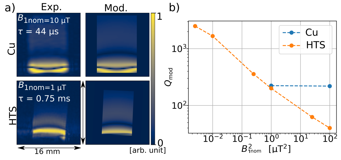
3D acquisitions of a 1 mL water sample were obtained at 1.5 T using a volume coil coupled during transmission and reception to different surface coil, in copper and in HTS³ material (YBa₂Cu₃O_7-δ), both with a diameter of 12 mm. Rectangular RF pulses were generated by the volume coil with $$$B_{1,\textrm{nom}}\in$$$ [0.05 μT, 10 μT] and pulse durations $$$\tau\in$$$ [6.4 μs, 4.0 ms]. Experimental results were adjusted to the model using a gradient descent algorithm where the fitting parameters were $$$\vec{r}_0$$$, $$$A$$$ and $$$Q_\textrm{mod}$$$ as defined earlier. The surface coils field maps $$$\vec{B}_1'$$$ were computed using the coils geometries and the Python library Magpylib⁴.

Results

Experimental results (Figure 1a-Exp.) are in good agreement with the computed ones (Figure 1a-Mod.). For all $$$B_{1,\textrm{nom}}$$$ amplitudes the $$$Q_\textrm{mod}$$$ values of the copper coil (222) determined by MRI are close to those measured with a network analyzer. In the case of the HTS material, the determined $$$Q_\textrm{mod}$$$ varies from 2500 to 50 for varying from 0.05 μT to 10 μT, also in good agreement with bench measurement results⁵.

Conclusions

The proposed model exploits the magnetic field map $$$\vec{B}_1'$$$ of a surface coil in order to determine its quality factor $$$Q$$$, and hence the intrinsic properties of the coil conductor in different experimental conditions (here the volume coil field amplitude). The $$$Q$$$ values determined with this model are of the same order of magnitude as the ones previously measured⁵. This method will allow for a better characterization of HTS coils functioning in MRI, as a function of $$$B_{1,\textrm{nom}}$$$ and of their working temperature $$$T$$$. This, in turn, will help design new HTS coil structures achieving better decoupling $$$(Q \to 1)$$$ when working with sufficiently strong $$$B_{1,\textrm{nom}}.$$$

Acknowledgements

Experiments were performed on the 1.5 T MRI platform of CEA/SHFJ, affiliated to the France Life Imaging network and partially funded by the network (grant ANR-11-INBS-0006).