Introduction

The low signal-to-noise ratio that is associated with magnetic resonance imaging (MRI) can be alleviated by a number of technical advancements, such as employing form-fitted phased array radio frequency (RF) coils. A novel realization of a flexible RF coil is the coaxial coil (CC) transmission line resonator (TLR), comprised of coaxial cable^1,2. The inner and outer conductor (cable shield), separated by a dielectric material and intersected by diagonally opposite gaps, are acting as the two transmission line segments. It is a self-resonant structure and its resonant frequency depends on coil geometry and material properties, such as coil diameter, dielectric permittivity and number of gaps. Although it seems natural to use such self-resonant coils at their resonance frequency, recent studies showed successful operation of a CC far away from their self-resonance employing capacitive and/or inductive tuning across the coil port³. In this work we investigate the performance of CCs at their self-resonance (f₀) as well as at the respective Larmor frequency (f_L) for 3T and 7T MRI employing 3D electromagnetic simulation.

Methods

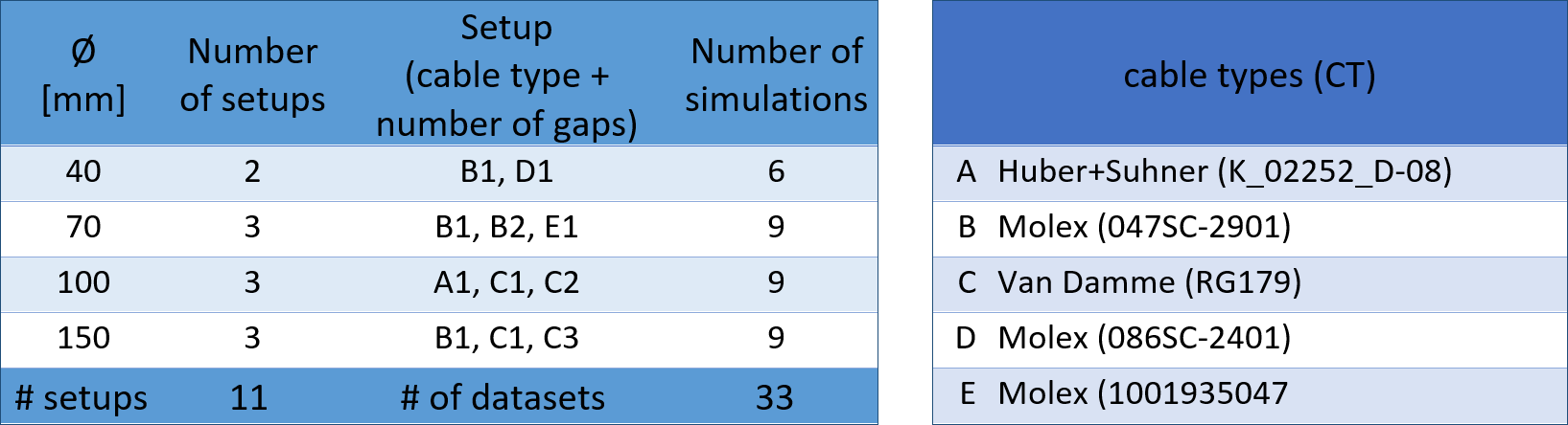
Eleven CC setups, differing in coil diameter (40,70,100 and 150mm), number of gaps (1-3) and cable type were modeled. Their performance in terms of their mean surface current amplitude at f₀ and f_L for Siemens 3T and 7T MRI systems, i.e. 123.3MHz and 297.2MHz, respectively, were investigated. The different setups are stated in more detail in Table 1.
Simulations were performed using the finite element solver of CST Studio Suite 2020 (Dassault Systèmes, Paris, France). Second order finite elements were used to approximate curved surfaces of the coaxial cable. Broadband results between 50 and 500MHz were generated using the general-purpose broadband sweep method of CST (maximum S-parameter interpolation error=0.001), using approximately 10 frequency samples. For each setup, f₀ of the unloaded coaxial loop was determined by finding the first local maximum of |Z|. 3D current monitors were then placed at f₀ and f_L for 3T and 7T. Surface current density ($$$K=dI/dl$$$) as well as the accepted power were exported for post-processing in Matlab 2017b (Mathworks, Natick, MA, USA). Simulations were scaled to 1W of actually accepted input power derived from simulation. The surface current density was analyzed on three conducting structures: the surface of the inner conductor (iC) and the inner and outer surface of the cable shield (oCi and oCo, respectively). The surface current I was derived by integrating K over volumes along the structures of a length of 1mm and multiplication with the respective conductor circumference.

Results and discussion

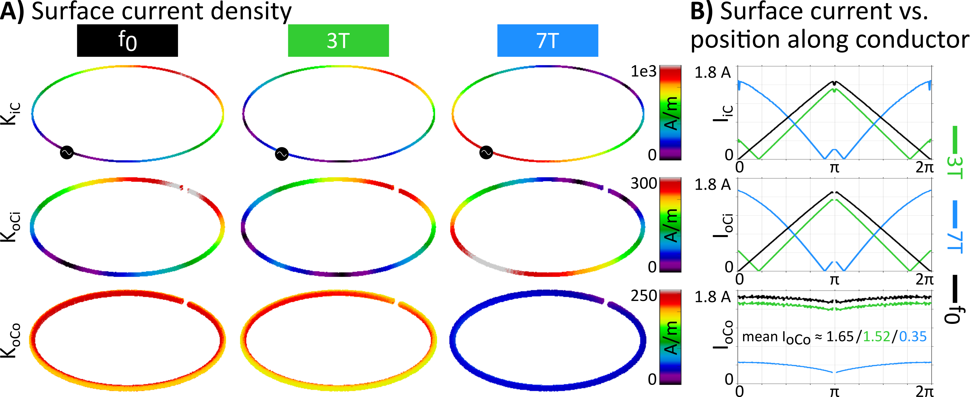
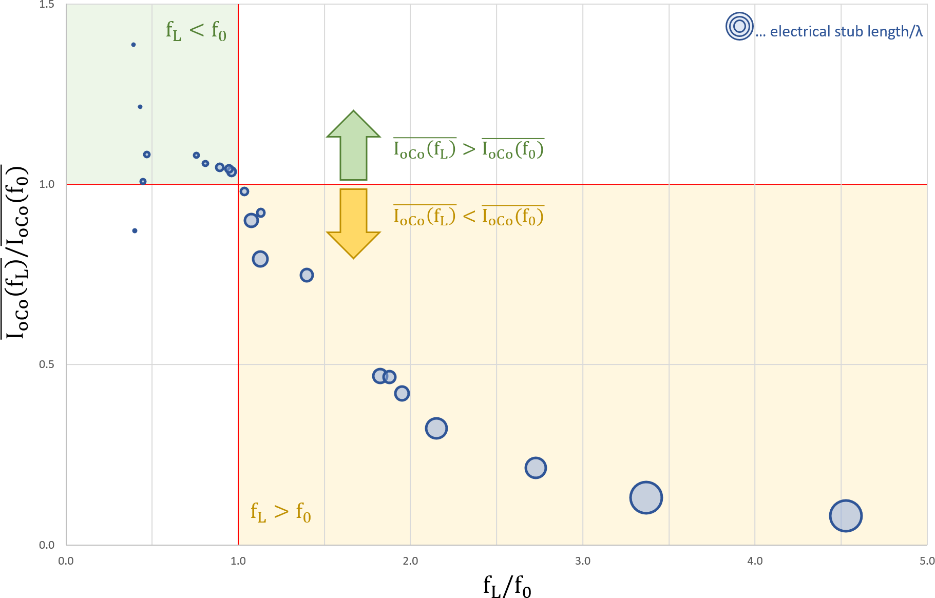
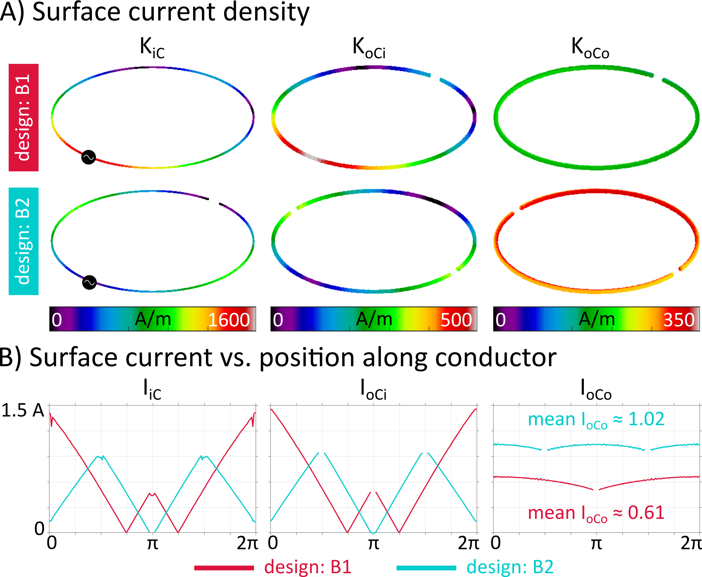
Generally, the current on oCi is the mirror-current with opposite direction of I on iC. At their respective f₀, the classical TLR behavior, i.e. a maximum in current density magnitude at each outer gap and a zero at each inner gap, can be observed. The current that effectively produces the B₁ field in the sample is the one running on oCo, is constant along the conductor as long as the segment length is electrically short versus the wavelength. Figure 1A shows an exemplary dataset (Ø=100mm, 1 gap, cable type A) of K on iC, oCi, and oCo evaluated at the 3 investigated frequencies. Figure 1B shows the corresponding I on the respective structures. We see that for 3T and f₀ (Fig.1B green and black line), the results are comparable, since f_L is close to self resonance (f_L/f₀≈1.13). Whereas for 7T (Fig.1B blue line), far away from self-resonance (f_L/f₀≈2.73) the surface current distribution is very different. The resulting mean surface currents on oCo ($$$\overline{I_{oCo}}$$$) near self-resonance are about a factor of 4-5 higher than for the 7T result operated far away from self-resonance. The performance of each coil design in terms of $$$\overline{I_{oCo}}$$$ when operated at one of the investigated Larmor frequencies ($$$\overline{I_{oCo}(f_L)}$$$) with respect to its performance at f₀ ($$$\overline{I_{oCo}(f_0)}$$$) is plotted versus the deviation of f_L from f₀ can be seen in Figure 2. For all investigated coils operated above their self-resonance, the ($$$\overline{I_{oCo}(f_L)}/\overline{I_{oCo}(f_0)}$$$) decreases with increasing ratio f_L/f₀ (see Fig.2 yellow area). For designs where this is not the case (f_L<f₀) no clear tendency could be identified. Most designs showed higher current (Fig.2 green area), whereas 2 designs showed equal or smaller current. Additionally, a trend for lower mean surface current with electrically longer segments between the gaps was observed. Figure 3 shows two coil designs evaluated at f_L=297.2MHz with the same diameter and cable type (Ø=70mm, cable type B) with 1 gap at 2.2 time the self-resonance frequency (B1) and with 2 gaps close to self-resonance (B2), f_L/f₀=1.1. The mean surface current for the coil approximately at self-resonance is ≈ 70% higher.

Conclusion

We were able to demonstrate that the mean surface current on the MR signal-relevant outer surface of the shield of coaxial coils decreases, the further above their self-resonance frequency they are operated. For operating frequencies below f₀, more datasets in that regime are needed to draw a conclusion. In this study, multi-gap designs with symmetric placement of gaps were investigated, in future studies also asymmetrical gap locations, as introduced by Mollaei et al.⁴, need to be taken into account. In future studies the resulting B₁⁺ and SAR will be investigated to obtain directly MR signal-relevant performance indicators.

Acknowledgements

This project was funded by the Austrian/French FWF/ANR grant, Nr. I-3618, “BRACOIL“