1399
Parametric Coil Optimization via Global Optimization
Jose EC Serralles1, Elfar Adalsteinsson2,3, Lawrence L Wald4, and Luca Daniel1
1Computational Prototyping Group (CPG), Research Laboratory of Electronics (RLE), Department of Electrical Engineering and Computer Science (EECS), Massachusetts Institute of Technology (MIT), Cambridge, MA, United States, 2Department of Electrical Engineering and Computer Science (EECS), Massachusetts Institute of Technology (MIT), Cambridge, MA, United States, 3Institute for Medical Engineering and Science (IMES), Massachusetts Institute of Technology (MIT), Cambridge, MA, United States, 4Martinos Center for Biomedical Imaging, Massachusetts General Hospital, Harvard Medical School, Boston, MA, United States
1Computational Prototyping Group (CPG), Research Laboratory of Electronics (RLE), Department of Electrical Engineering and Computer Science (EECS), Massachusetts Institute of Technology (MIT), Cambridge, MA, United States, 2Department of Electrical Engineering and Computer Science (EECS), Massachusetts Institute of Technology (MIT), Cambridge, MA, United States, 3Institute for Medical Engineering and Science (IMES), Massachusetts Institute of Technology (MIT), Cambridge, MA, United States, 4Martinos Center for Biomedical Imaging, Massachusetts General Hospital, Harvard Medical School, Boston, MA, United States
Synopsis
Algorithmic design of coil arrays in MRI is typically considered desirable but computationally intractable. In this work, we demonstrate that it is in fact feasible to programmatically optimize over the design of a coil array to achieve a metric-of-interest, such as slice homogeneity in the transmit field. We build on previous work by employing global optimizers in several of the key steps in the optimization procedure. We demonstrate the effectiveness of this approach via a couple of numerical examples.
Introduction
The increase in Larmor frequency over the years in MRI has yielded a number of benefits, such as lower acquisition time and increased parallelization. However, it has also presented a number of drawbacks, such as the need for strict SAR constraints, greater difficulty in the design of coil arrays, and more complicated and slower simulation approaches.[1] In this work, we demonstrate that it is in fact feasible to employ an algorithmic approach when designing the parameters of a coil array. We build on previous work [2] by employing global optimization strategies that increase the robustness of our solutions and indeed improve the performance gains that we observe.Methods
We pose the parametric design of the coil array as an optimization problem,$$\min_{R,C,\alpha}\|H^+(R,C,\alpha)-\hat{h}^+\|_2^2\\
\text{s.t. tuning, matching & shimming}$$
which minimizes the discrepancy between a desired transmit field $$$\hat{h}^+$$$, homogeneous on a central slice in the head, and the field $$$H^+(R,C,\alpha)$$$, produced by an array of coils with geometry parameters $$$R$$$, capacitor values $$$C$$$, and shimming coefficients $$$\alpha$$$.
In practice, we decompose the optimization into an outer loop which iterates only over the geometric parameters, and two inner loops for tuning & matching as well as shimming. Figure 1 shows a graphical representation of our proposed procedure. More specifically, in each of the outer loop iteration we take a new guess at the geometry (i.e. parameter $$$R$$$). We then solve a first inner optimization $$$\min_C{\|S(C)\|_F^2}$$$ to find capacitor values $$$C$$$ by enforcing tuning & matching on the scattering parameter matrix $$$S$$$. We precede tuning and matching with a global optimization that finds first a rough guess for capacitor values.
Finally, we find optimal shimming coefficients $$$\alpha$$$ solving a second inner optimization $$$\min_{\alpha}{\|H^+(\alpha)-\hat{h}^+\|_2^2}$$$ where $$$H^+(\alpha)$$$ is the field resulting from the superposition of the fields produced by the individual coils in the array.
Materials
We use the open-source meshing software package gmsh [3] to design a loop and obtain a template mesh. We use the Magnetic Resonance Integral Equation (MARIE) suite [4], i.e. an integral equation-powered simulation tool that uses RWG basis functions in a surface integral formulation for the coil currents and volumetric currents for the body. We employ the Magnetic Resonance Green's Function (MRGF) approach [5], which allows pre-computation of the body-body interactions. As body model, we use the Billie Head Model from the Virtual Family [6], which supplies us with a voxelized representation of the permittivity $$$\epsilon$$$ and conductivity $$$\sigma$$$ at a $$$B_0$$$ static field strength of 7 Tesla.Numerical Experiments
We ran a series of numerical experiments using a loop parameterized by its radius $$$R$$$ and the Billie head phantom at 7 Tesla:In the first experiment, we placed two coils to the left and to the right of the head. Both coils had initial radii of 9 cm, yielding an initial cost function value of 250. After 251 iterations of the outer loop or 8 hours of runtime, we found the optimal radii to be 12 cm on the left and 8.6 cm on the right, yielding a final cost function value of 19.5, or roughly $$$12\times$$$ reduction in inhomogeneity. Figure 2 compares the initial and final setups and their respective fields.
In the second experiment, we placed two coils in the front and the back of the head. Each coil had an initial radius of 11.5 cm, with an initial cost function value of 155. After 750 iterations of the outer loop or 5.4 hours, we found the optimal radii to be 9.17 cm on the front and 11.2 cm on the back, with a final cost function value of 69.7, or roughly $$$2.2\times$$$ reduction in inhomogeneity. Figure 3 compares the initial and final setups and their respective fields.
In the third experiment, we placed four coils around the head. Each coil had an initial radius of 9 cm, yielding an initial cost function value of 128.4. After 332 iterations or 8 hours, we found the optimal radii to be 11.7, 12.0, 7.2, and 9.6 cm with a final cost function value of 19.9 or a $$$6.43\times$$$ reduction in inhomogeneity. Figure 4 compares the initial and final setups and their respective fields.
Discussion & Conclusion
All three experiments resulted in significantly more homogeneous fields, with the minimum attainable cost function value to be approximately 20. The runtime of experiment 1 was considerably higher per iteration because the computing resources were under heavy load, and we estimate that its runtime should have been roughly 1.8 hours. Interestingly, the addition of the two coils in the front and back seems to have been inconsequential to homogeneity, as the final cost function in Exp. 1 was 19.5 and in Exp. 3 was 19.9. Additionally, when only the front and back loops are used in Exp. 2, the minimum cost function value was 69.7. We hypothesize that this might be due to the front and back being farther away from the centroid of the head. Further investigation would be necessary to discern which of these hypotheses is correct. We can conclude that our simulation and optimization approaches render the algorithmic design problem feasible, reliable, and effective.Acknowledgements
This work was supported by NIH 2R01EB006847-09A1.References
- Fagan, A. J., Bitz, A. K., Björkman‐Burtscher, I. M., Collins, C. M., Kimbrell, V., Raaijmakers, A. J., & ISMRM Safety Committee. (2020). 7T MR Safety. Journal of Magnetic Resonance Imaging.
- J.E.C. Serralles et al. Rapid parametric optimization of transmit coil arrays: a proof-of-concept. (2020) ISMRM 2020, p. 4262.
- C. Geuzaine and J.-F. Remacle. Gmsh: a three-dimensional finite element mesh generator with built-in pre- and post-processing facilities. International Journal for Numerical Methods in Engineering 79(11), pp. 1309-1331, 2009.
- J. F. Villena et al., “MARIE–a Matlab-based open source software for the fast electromagnetic analysis of mri systems,” in Proceedings of the 23rd Annual Meeting of ISMRM,. ISMRM Toronto, Canada, 2015, p.709.
- J. F. Villena et al., "Fast Electromagnetic Analysis of MRI Transmit RF Coils Based on Accelerated Integral Equation Methods," in IEEE Transactions on Biomedical Engineering, vol. 63, no. 11, pp. 2250-2261, Nov. 2016, doi: 10.1109/TBME.2016.2521166.
- Christ, Andreas, et al. "The Virtual Family—development of surface-based anatomical models of two adults and two children for dosimetric simulations." Physics in Medicine & Biology 55.2 (2009): N23.
- Steven G. Johnson, The NLopt nonlinear-optimization package, http://github.com/stevengj/nlopt
- D. R. Jones, C. D. Perttunen, and B. E. Stuckmann, "Lipschitzian optimization without the lipschitz constant," J. Optimization Theory and Applications, vol. 79, p. 157 (1993).
- S. Gudmundsson, "Parallel Global Optimization," M.Sc. Thesis, IMM, Technical University of Denmark, 1998.
Figures
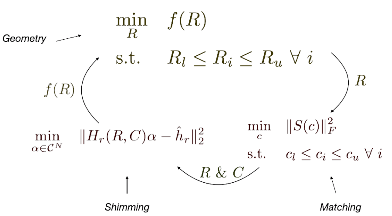
A visual representation of the coil optimization procedure.
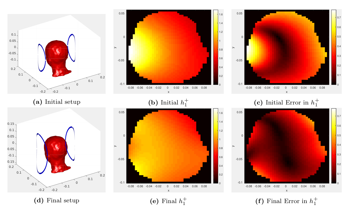
Experiment 1, with coils to the left and right. Figs. a and d show the initial and final setups, respectively. Figs. b and e show the initial and final transmit magnetic fields. Figs. c and f show the difference between the transmit fields and the desired fields.

Experiment 2, with coils in the front and back. Figs. a and d show the initial and final setups, respectively. Figs. b and e show the initial and final transmit magnetic fields. Figs. c and f show the difference between the transmit fields and the desired fields.
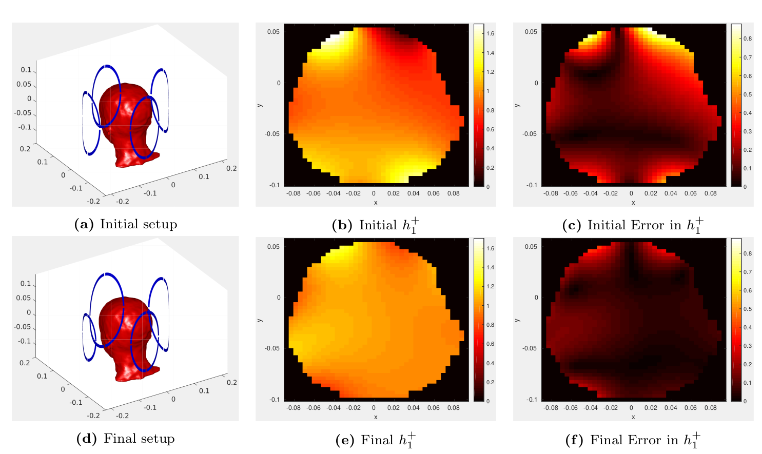
Experiment 3, with coils around the head phantom. Figs. a and d show the initial and final setups, respectively. Figs. b and e show the initial and final transmit magnetic fields. Figs. c and f show the difference between the transmit fields and the desired fields.