1389
Detection of Head Motion using Navigators and a Linear Perturbation Model
Thomas Ulrich1 and Klaas Paul Pruessmann1
1Institute for Biomedical Engineering, ETH Zurich and University of Zurich, Zurich, Switzerland
1Institute for Biomedical Engineering, ETH Zurich and University of Zurich, Zurich, Switzerland
Synopsis
We propose a novel algorithm for motion estimation with k-space navigators. The algorithm operates on the complex k-space navigator signal. It uses a linear signal model, which describes how the navigator signal changes under rotation and translation of the imaged object. Rotation and translation are estimated simultaneously by means of linear least-squares parameter fitting using the linear model. We show that the algorithm achieves high accuracy and precision through a phantom experiment with a motionless phantom. Furthermore, we show the algorithms's applicability in-vivo during a volunteer experiment with and without intentional head motion.
Introduction
Patient motion is one of the leading causes of image artifacts in MR imaging. Many different methods for motion correction have been developed during the last few decades.1-3 K-space navigators are a particularly promising approach, because they are a purely MR-signal-based approach that does not require any additional hardware. We propose a novel algorithm for navigator-based motion estimation that uses a linearized perturbation model of complex-valued signal changes for estimating rotations and translations with high accuracy and low computational complexity.Methods
We inserted a navigator readout into a 3D-FFE sequence during the dead time between excitation and phase-encoding (Figure 1). The first navigator signal is used to calculate a matrix M based on a linear perturbation model, which is described below. All other navigator signals are used for motion estimation using the matrix M.Theory
Rotations of an imaged object rotate the k-space signal accordingly, while translations lead to a linear phase shift on the signal. Formally, if we denote by $$$s(k(t))$$$ and $$$\tilde{s}(k(t))$$$ the k-space signal of an object before and after applying a 3x3 rotation matrix $$$R(\theta)$$$ and a 3D shift vector $$$\Delta x$$$, then:
$$\tilde{s}(k(t))=s(R(\theta)k(t))e^{i\Delta x^Tk(t)}$$
If the rotation angles and translation vector are small, the above equation can be approximated by a first-order Taylor expansion, which can be written as linear function of the angles and shift. This assumption is usually satisfied if the navigator radius is chosen small enough, so that the absolute displacements $$$R(\theta)k(t)-k(t)$$$ of the trajectory are just a fraction of the Nyquist interval.
$$\tilde{s}(k(t))-s(k(t))=\sum_{d=1}^3\frac{\mathrm{d}s}{\mathrm{d}\theta_d}\theta_d+i\Delta x^Tk(t)s(k(t))$$
The derivatives $$$\frac{\mathrm{d}s}{\mathrm{d}\theta_d}$$$ can be calculated using the chain rule of differentiation:
$$\frac{\mathrm{d}s}{\mathrm{d}\theta_d}=\frac{\partial s(k)}{\partial k}\left.\frac{\partial R(\theta)}{\partial \theta_d}\right\vert_{\theta_d=0}k(t)$$
The rotational displacement $$$\left.\frac{\partial R(\theta)}{\partial \theta_d}\right\vert_{\theta_d=0}k(t)$$$ can be split into a tangential component of the k-space trajectory (a multiple of $$$\dot{k}(t)$$$), and a component which is orthogonal to $$$\dot{k}(t)$$$. The derivative of the signal in the tangential direction is given by $$$\dot{s}(t)$$$. Calculating the derivative in any direction orthogonal to $$$\dot{k}(t)$$$, however, would require k-space data from an area of k-space, that is not covered by the navigator trajectory. Therefore, we only consider the tangential component of the derivative $$$\frac{\mathrm{d}s}{\mathrm{d}\theta_d}$$$, and denote it by $$$\eta_d$$$:
$$\eta_d(t)=\frac{\dot{s}(t)}{\Vert\dot{k}(t)\Vert^2}\left\langle \left.\frac{\partial R(\theta)}{\partial \theta_d}\right\vert_{\theta_d=0}k(t),\dot{k}(t) \right\rangle$$
Since the measurement noise on the complex-valued navigator signals follows a zero-mean Gaussian distribution, we calculate the angles $$$\theta$$$ and shift vector $$$\Delta x$$$ by linear least-squares estimation. The spectrometer samples the MR signal only at discrete timepoints $$$t_1,t_2,\dots$$$. Therefore, we need to write our estimation problem in matrix-vector form. We define the following matrix M, which relates rotation angles and shifts to signal perturbations.
$$M=\begin{pmatrix}ik_1(t_1)s(k(t_1))&ik_2(t_1)s(k(t_1))&ik_2(t_1)s(k(t_1))&\eta_1(t_1)&\eta_2(t_1)&\eta_3(t_1)\\ik_1(t_2)s(k(t_2))&ik_2(t_2)s(k(t_2))&ik_2(t_2)s(k(t_2))&\eta_1(t_2)&\eta_2(t_2)&\eta_3(t_2)\\\vdots&\vdots&\vdots&\vdots&\vdots&\vdots\\ik_1(t_n)s(k(t_n))&ik_2(t_n)s(k(t_n))&ik_2(t_n)s(k(t_n))&\eta_1(t_n)&\eta_2(t_n)&\eta_3(t_n)\end{pmatrix}$$
If we stack the sampled MR signal into column vectors $$$s,\tilde{s}$$$, we can solve the linear least-squres problem by multiplication of the signal vectors and the Moore-Penrose pseudoinverse of M:
$$\begin{pmatrix}\Delta x\\\theta\end{pmatrix}=M^\dagger(\tilde{s}-s)$$
Experiments
All experiments were performed at a 7T Philips Achieva scanner using a 32-channel head coil. We used a single-shot 3D orbital navigator4, which is displayed in Figure 2.
To examine the precision of the method, a motionless phantom (pineapple) was placed in the head coil. Navigator signals were acquired during a 3D T2*w-FFE imaging scan and motion parameters were estimated from the navigator signal.
We also performed two in-vivo experiments. For the first experiment, a volunteer was instructed to hold still during a 2.5-minute FFE scan sequence. During the second experiment, the volunteer was instructed to move their head around all six degrees of freedom. Motion parameters were estimated using our proposed algorithm.
Results
Figure 3 shows the results from the experiment with the motionless phantom. The algorithm produced rotation angles in the range of ±0.15 degrees and shifts in the range of ±60μm, with root-mean squares values of up to 0.04 degrees and 25μm.Figures 4 and 5 show the estimated rotation angles and shifts from the two in-vivo experiments. During the experiment without intentional motion, the rotation was estimated to be within the range of ±0.2 degrees and ±0.25mm, except for the HF axis, where the estimated shift values seem to drift and oscillate around -0.2mm. The spectrum showed distinct peaks at 0.30 Hz and 1.22 Hz.
When the volunteer moved intentionally, rotation angles of up to ±2 degrees and shifts of ±3.5mm were reported by our algorithm.
Discussion
The phantom experiment demonstrates that our method exhibits high precision and accuracy. Since we know that no actual object motion has occurred, we can conclude that our method's estimates were correct up to the RMS error of 0.04 degrees and 25μm, and the standard deviation is of roughly the same size.In case of the in-vivo experiment, no ground truth is available, unfortunately. However, the results indicate that our algorithm is sensitive to head motion. The peaks in the spectrum at 0.30 Hz and 1.22 Hz are likely due to respiration and heartbeat. Further investigation of the accuracy and precision for head motion estimation is to be conducted in the future.
Conclusion
We have demonstrated that rigid-body motion can be accurately and precisely characterized using our motion estimation algorithm. The navigator readout is very fast and the algorithm has very low computational complexity, so the motion parameters can be calculated within milliseconds.Acknowledgements
No acknowledgement found.References
- Zaitsev Maxim, Maclaren Julian & Herbst Michael. Motion artifacts in MRI: A complex problem with many partial solutions. Journal of Magnetic Resonance Imaging 42, 887–901 (2015).
- Godenschweger, F. et al. Motion correction in MRI of the brain. Phys. Med. Biol. 61, R32 (2016).
- Maclaren, J., Herbst, M., Speck, O. & Zaitsev, M. Prospective motion correction in brain imaging: A review. Magnetic Resonance in Medicine 69, 621–636 (2013).
- Ulrich, T., Patzig, F., Wilm, B. J. & Pruessmann, K. P. Towards Optimal Design of Orbital K-Space Navigators for 3D Rigid-Body Motion Estimation. ISMRM & SMRT Virtual Conference & Exhibition (2020).
Figures
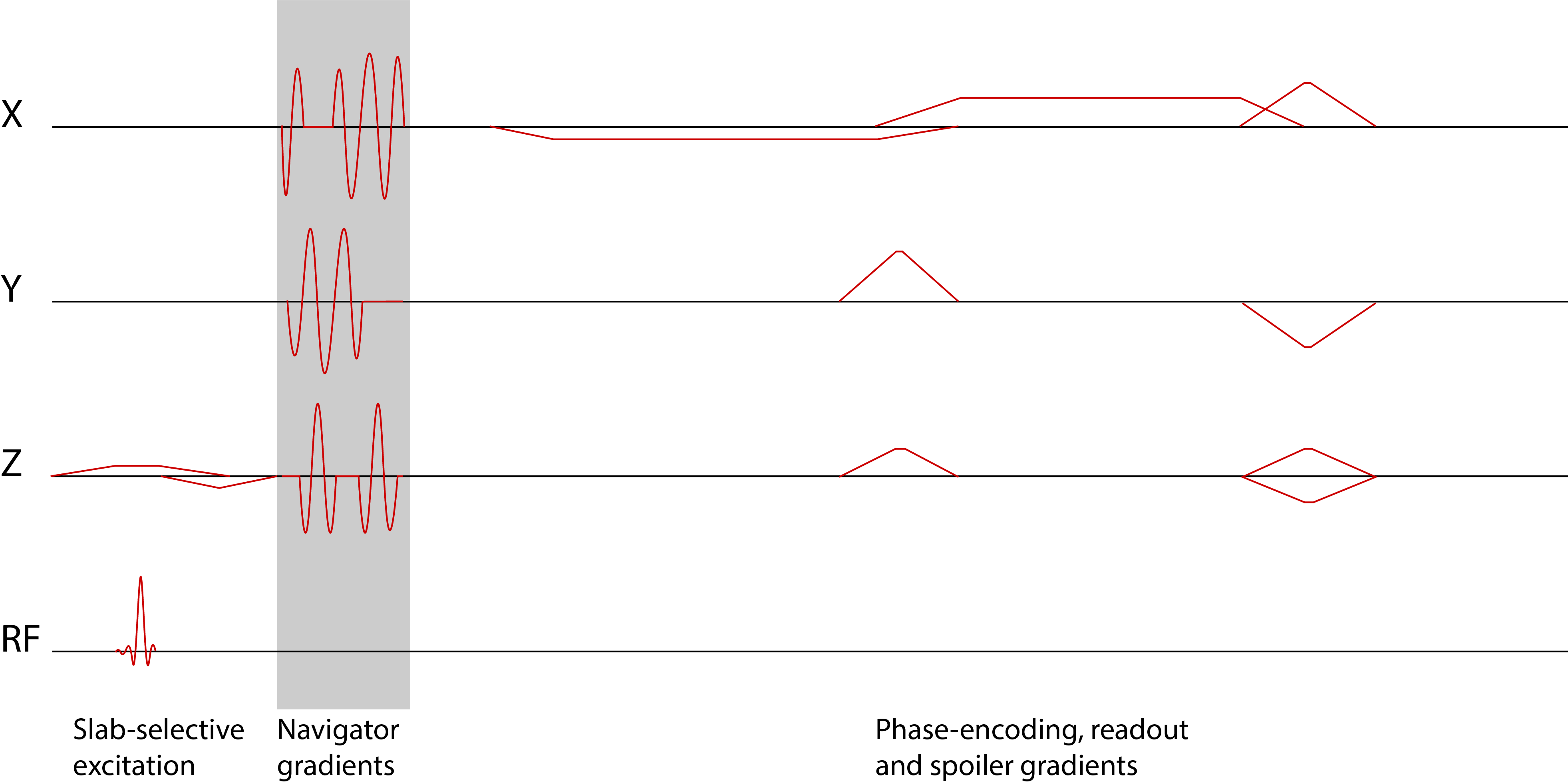
Sequence diagram of a 3D T2*-weighted FFE sequence with 3D orbital navigator gradients inserted after the excitation and before the phase-encoding gradients.
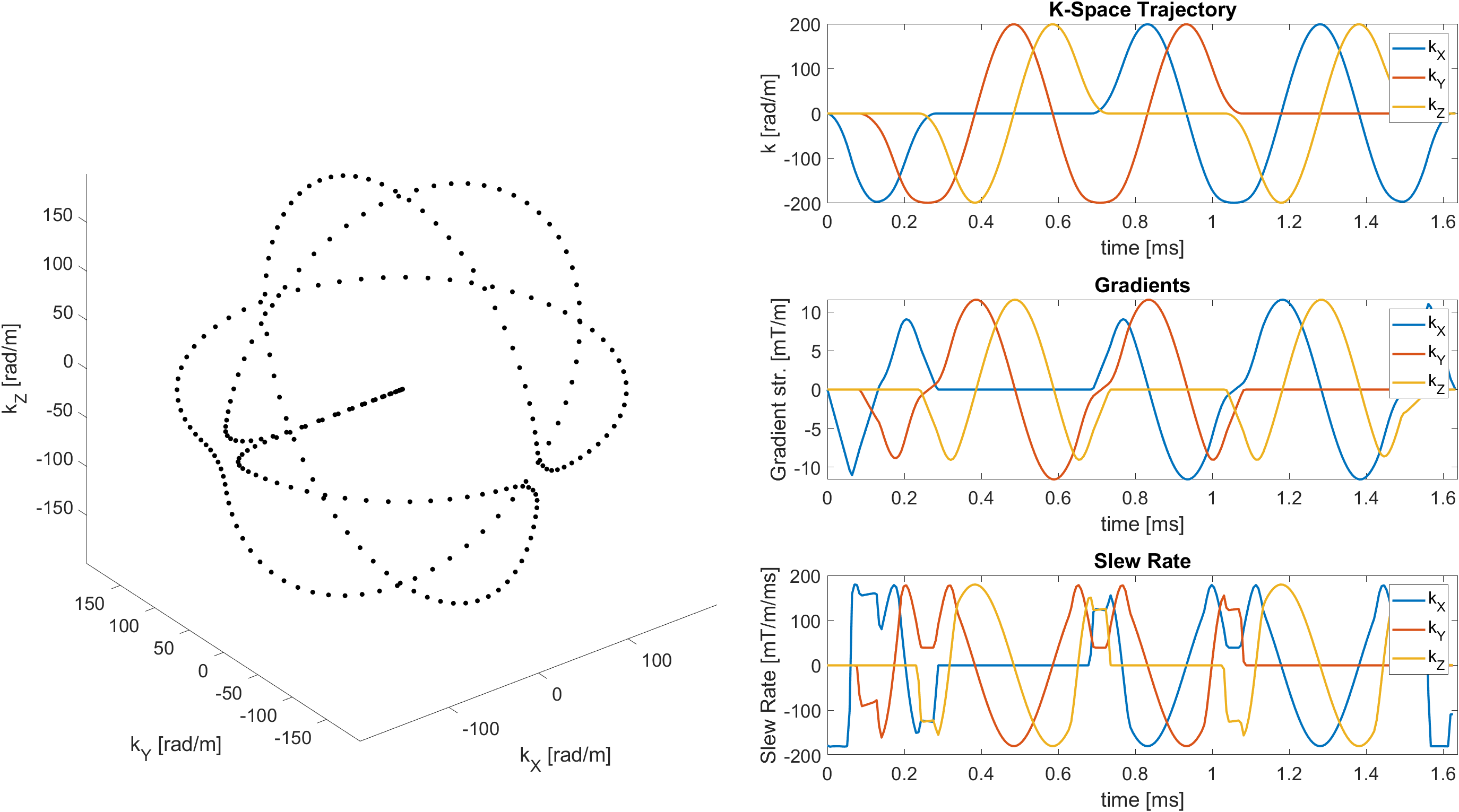
Orbital navigator k-space trajectory. Left: Parametric plot of the trajectory shape. Right: Plots of the trajectory, gradients, and slew rate over time. The trajectory is made up of three orthogonal circles, with smooth transitions in between them. At a radius of 200 rad/m, the navigator gradients can be executed in about 1.65 milliseconds.
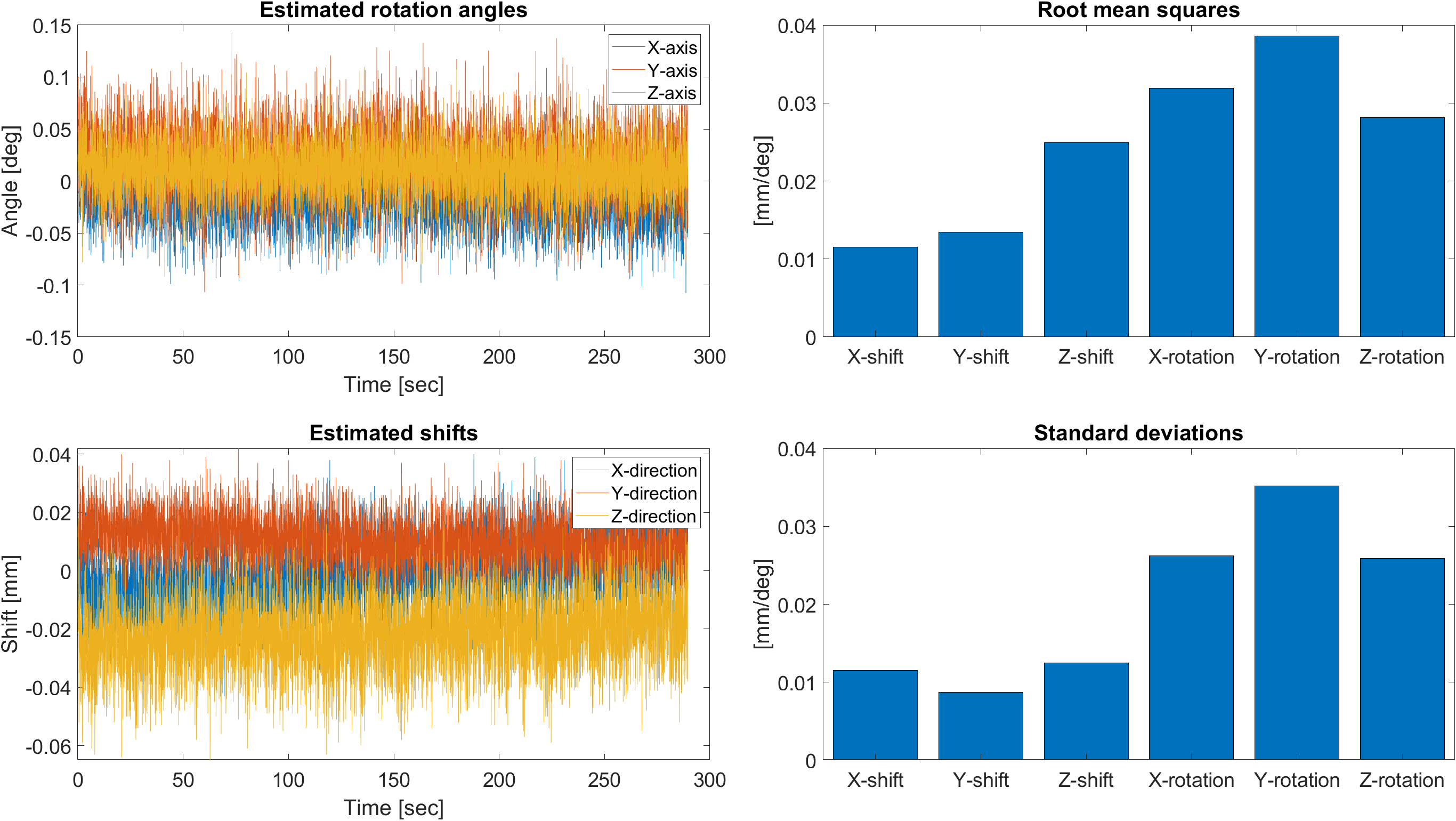
Left: Estimated rotation angles and translational shift from an experiment with a motionless phantom (pineapple). Right: Standard deviation and root mean squares of the rotation angles and translation parameters over time.
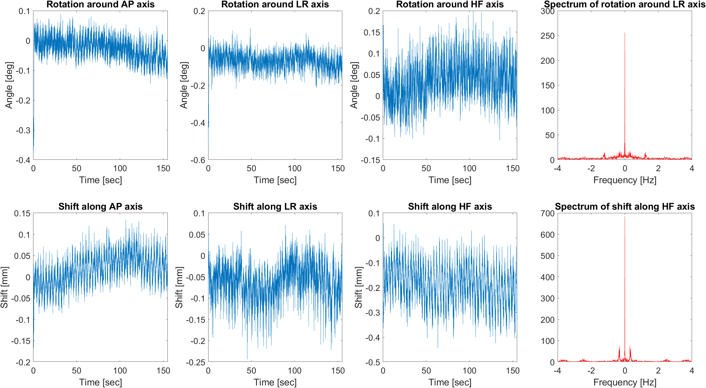
First three columns: Estimated motion parameters from an in-vivo experiment where the volunteer was instructed to hold still. Fourth column: Spectra of the motion time series of two selected axes. Rotations around the LR axis show a peak in the spectrum at 1.22 Hz, shifts along the HF axis at 0.30 Hz.
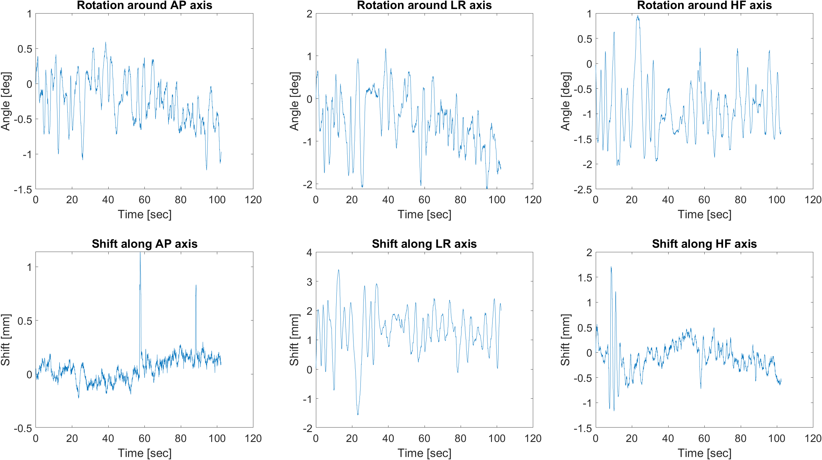
Estimated motion parameters from an in-vivo experiment where the volunteer was instructed to move their head around randomly around all six degrees of freedom.