Introduction

Head motion during image acquisition causes artefacts. These artefacts can be eliminated by using motion correction techniques based on tracking head pose using markers that are attached to the head ^{1, 2, 3}. Here we use simulations to evaluate the feasibility of a novel approach to motion tracking, which is based on using a 16-probe field camera to monitor the fields generated by briefly passing currents through small coils affixed to the head. The benefits of this approach are that problematic line-of-sight access to markers is not required (cf. optical approaches) and that it could be implemented without modification of the MRI sequence (cf. navigators).

Methods

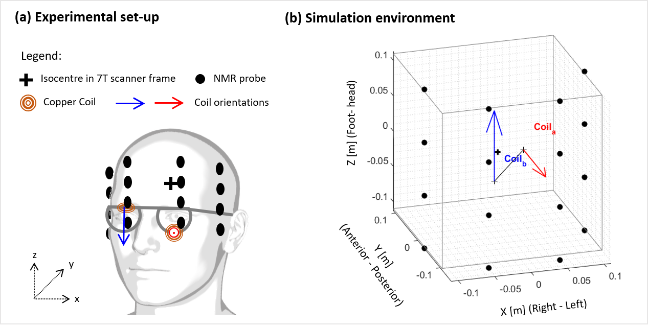
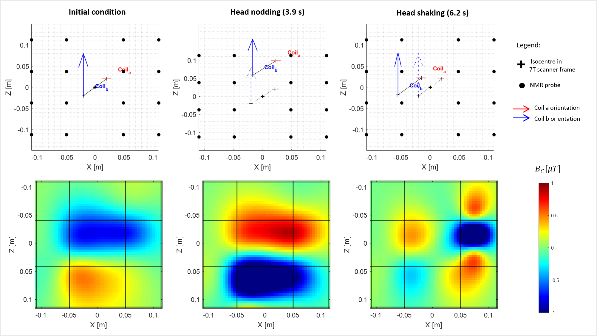
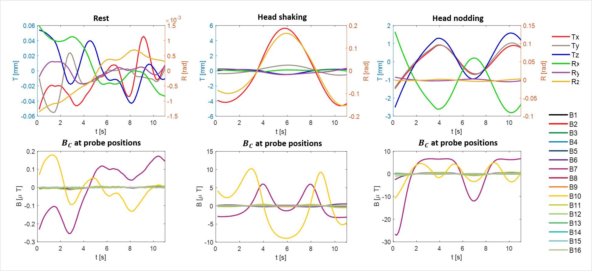
The simulated set-up is shown in Figure 1. Two, small solenoidal coils (100 turns; i.d. 5.2mm; o.d. 10.2mm; 2.5mm length) were positioned on the end-pieces of a pair of glasses. The two coils’ orientations were chosen to be approximately along the y- and z-axes. The z-component of the magnetic field from the coils is monitored using 16-field probes distributed over the upper part of the internal surface of the Tx RF coil. The magnetic fields generated at the fixed probe positions were calculated for each head position using analytic expressions for the field from solenoidal coils carrying a current of 0.3 A ⁴. Figure 2 shows the Bz-field generated at the probe-surface for one head pose, and the field-changes resulting from head pose changes during head nodding and head shaking.
To test the feasibility of tracking head motion using this approach, we simulated a time series (0.15s time-step) of field values produced at the probes (B_C(t)) using head motion parameters measured previously during motion correction experiments using an MPT optical camera^5,6. The motion parameter set (M(t)) characterises translations and rotations related to Cartesian axes in the scanner’s frame of reference. Motion parameters were then estimated from the 16 field-values recorded at each time point using the analytic field expressions. The prediction was performed using a Matlab function based on the Nelder-Mead Simplex optimization method⁶. The magnetic field change between consecutive time steps was used as the cost function. Given the value of the magnetic field at step n (B_C(t_n)), the value of the magnetic field at time t_n+1 is estimated by iteratively changing the motion parameters used to move the coil system and evaluating the magnetic field, B_P(t_n+1). The algorithm converges to the predicted motion parameters (M_p(t_n)) once the difference between the measured and estimated magnetic field changes reaches a fixed tolerance. The algorithm needs a starting guess for the motion parameters set (M₀(t_n)). For the first time step, M₀(t_n=1) was randomly extracted from a normal distribution with zero mean and deviation standard equal to the standard deviation of the motion parameters. For each subsequent time step, (M₀(t_n>1)), the guess was formed using a perturbation extracted in the same way, but scaled by 0.01, which was added to the previous prediction (M_p(t_n-1)). We also evaluated the effect of adding white noise (10^-9T std) to the simulated fields. Figure 3 shows the temporal variation of the motion parameter and simulated field values for 10s periods during rest, head-nodding and head-shaking conditions.

Results

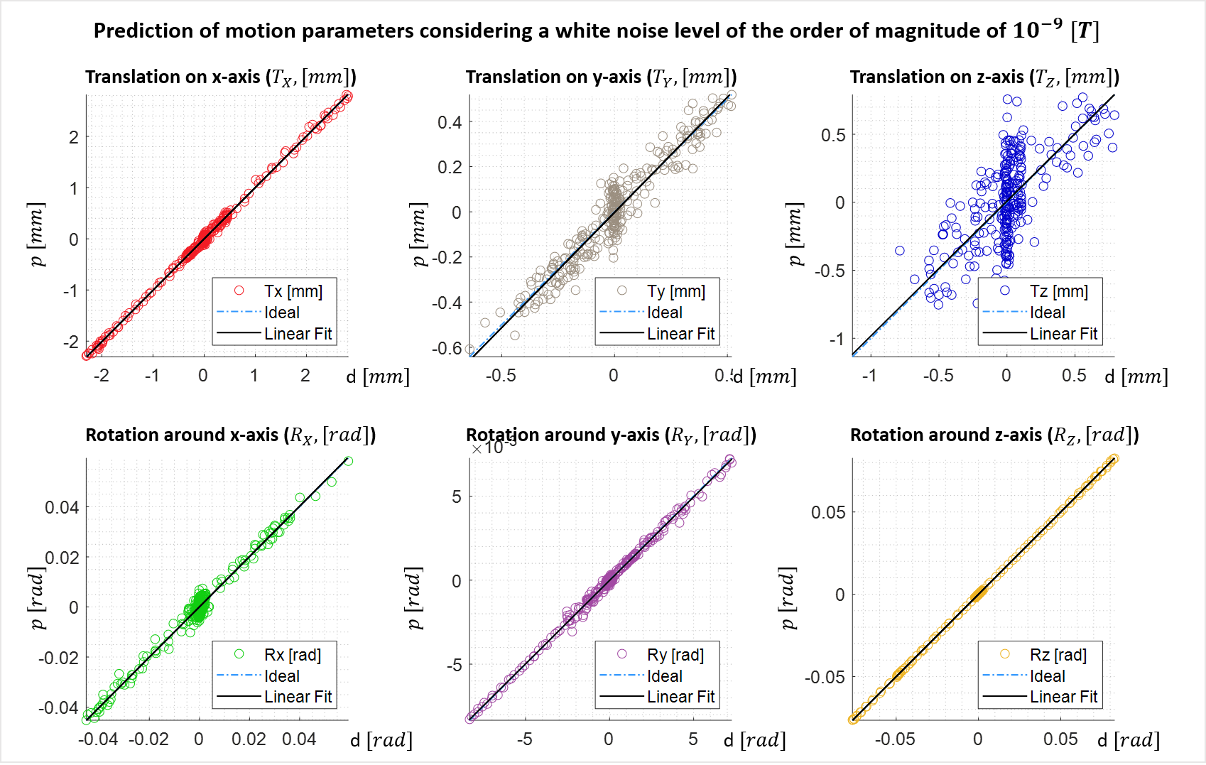
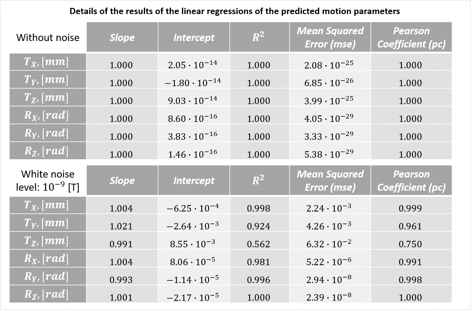
The prediction of motion parameters from the simulated field changes was performed on 300 data points (spanning 45 s) for each movement condition. The resulting motion parameter predictions collated from all three conditions are shown in Figure 4 for data with added noise. The predicted values for each motion parameter p have been plotted against the actual data values d: ideal prediction results would follow a straight line with unit slope. Table 1 details the results of a linear regression of the predicted motion parameters to the actual values (slope, intercept, R², the mean squared error (mse), and the Pearson coefficient (pc)).

Discussion

There is very good agreement between the predicted values for all motion parameters, indicating that head motion can be tracked using the combination of two coils and 16 field probes. The best results are obtained for rotations while translation in z is least accurately estimated. The first few predictions are most influenced by the initial random guess (M₀(t_n=1)) leading to greater prediction inaccuracy. The accuracy of the prediction is dictated by the choice of the stopping criteria of the algorithm and by the noise level. Inclusion of additional coils, which could be pulsed in combination with or, separately to, the initial coil pair would help to improve the localisation accuracy.

Conclusions

Head motion can be tracked by monitoring the fields produced by small coils attached to the head using a field camera. The good prediction accuracy achieved using simulated data indicate that it is worth implementing this approach experimentally to provide a marker-based motion correction technique that does not require line-of-sight access or significant modification of the image acquisition. This will require synchronisation of coil pulsation and field measurement with ‘quiet’ periods of the sequence and minimisation of RF and B₀ field interactions with the coils.

Acknowledgements

No acknowledgement found.