INTRODUCTION

MHD flow is a phenomenon that emerges inside the conductive fluids due to the orthogonal magnetic field and electrical current density distributions. For instance, during Magnetic Resonance Current Density Imaging (MRCDI), an external current is injected into the medium.¹ The current density creates a Lorentz force density distribution by interacting with the static magnetic field of the MR scanner ($$$B_0$$$). As a result, fluid flow is introduced in compliance with the Navier-Stokes equations called MHD flow.² Furthermore, MHD is a well-known effect observed during an electrocardiogram (ECG) triggered MRI scans and has been reported to interfere with the measured ECG signal.^3,4 Consequently, MHD flow velocimetry is a novel and clinically important research problem. There are several studies that propose spin echo (SE) or gradient echo (GE) based pulse sequences with flow-encoding gradients to obtain MHD flow.^5-8 In these studies, the flow-encoding gradients are applied in one of the orthogonal directions (x-, y-, or z-) to measure the flow in that direction by encoding it into the MR signal phase. However, this choice of flow-encoding directions is not obligatory. With a different set of flow-encoding directions, the associated MR magnitude images can be utilized to obtain the diffusion tensor $$$\overline{\overline{D}}$$$) of the medium.

To obtain MHD flow velocity in three directions, twelve acquisitions in the presence of flow-encoding gradients and current injection must be conducted. The weighted average of four phase images having flow encoding in a specific direction gives the MHD flow in that direction. With the proposed set of the flow-encoding directions, it is also possible to extract $$$\overline{\overline{D}}$$$ from the associated MR magnitude images provided that at least one T₂-weighted image is acquired from the same region.
In this study, MHD flow and $$$\overline{\overline{D}}$$$ distributions obtained from the same measurements are demonstrated.

METHODS

The MR phase component formed due to MHD flow ($$$\phi_{MHD_{\mathbf{G_f}}}$$$) can be obtained as⁷:

$$\phi_{MHD_{\mathbf{G_f}}}=\frac{arg(S^{I_+\mathbf{G_f}_+})-arg(S^{I_-\mathbf{G_f}_+})-arg(S^{I_+\mathbf{G_f}_-})+arg(S^{I_-\mathbf{G_f}_-})}{4}\quad\quad\quad\quad\quad(1)$$

$$$S^{I_\pm\mathbf{G_f}_\pm}$$$ are the MR signal distributions with opposing flow-encoding gradients ($$$\mathbf{G_f}$$$) and injected current ($$$I$$$) polarities.

The relation between $$$\phi_{MHD_{\mathbf{G_f}}}$$$, the MHD flow velocity distribution ($$$\mathbf{v}$$$) and $$$\mathbf{G_f}$$$ can be formed as:


$$\phi_{MHD_{\mathbf{G_f}}}=-\int_{t_0}^{t_0+\delta}\gamma(\mathbf{G_f}\cdot\mathbf{v})dt+\int_{t_0+\Delta}^{t_0+\Delta+\delta}\gamma(\mathbf{G_f}\cdot\mathbf{v})dt=\gamma\delta\Delta(\mathbf{G_f}\cdot\mathbf{v})\quad\quad\quad\quad\quad(2)$$

where $$$\delta$$$ is the flow-encoding gradient duration, and $$$\Delta$$$ is the time interval between the starting points of two consecutive flow-encoding gradients. Hence, using the relation constructed in Equation 2, $$$\mathbf{G_f}$$$ can be used to compute $$$\mathbf{v}$$$ in the direction of $$$\mathbf{G_f}$$$.

If the flow encoding gradient vector directions are chosen carefully, with twelve measurements (6 with positive current polarity and 6 with the negative), both $$$\overline{\overline{D}}$$$, and MHD related phase distribution ($$$\phi_{MHD_{\mathbf{G_f}}}$$$) can be obtained separately. The conventional flow-encoding gradient set ($$$\mathbf{G_f^k}$$$) utilized in MHD measurements can be shown as^7,8:

$$\mathbf{G_f^1}=\begin{bmatrix}G_f\\0\\0\end{bmatrix},\mathbf{G_f^2}=\begin{bmatrix}-G_f\\0\\0\end{bmatrix},\mathbf{G_f^3}=\begin{bmatrix}0\\G_f\\0\end{bmatrix},\mathbf{G_f^4}=\begin{bmatrix}0\\-G_f\\0\end{bmatrix},\mathbf{G_f^5}=\begin{bmatrix}0\\0\\G_f\end{bmatrix},\mathbf{G_f^6}=\begin{bmatrix}0\\0\\-G_f\end{bmatrix}\quad\quad\quad\quad\quad(3)$$

On the other hand, the proposed set ($$$\mathbf{{G_f^k}^*}$$$) is given in Equation 4:

$$\mathbf{{G_f^1}^*}=\begin{bmatrix}G_f\\0\\G_f\end{bmatrix},\mathbf{{G_f^2}^*}=\begin{bmatrix}-G_f\\0\\G_f\end{bmatrix},\mathbf{{G_f^3}^*}=\begin{bmatrix}G_f\\G_f\\0\end{bmatrix},\mathbf{{G_f^4}^*}=\begin{bmatrix}G_f\\-G_f\\0\end{bmatrix},\mathbf{{G_f^5}^*}=\begin{bmatrix}0\\G_f\\G_f\end{bmatrix},\mathbf{{G_f^6}^*}=\begin{bmatrix}0\\G_f\\-G_f\end{bmatrix}\quad\quad\quad\quad\quad(4)$$
The main point here is that $$$\overline{\overline{D}}$$$ cannot be reconstructed with the set in Equation 3 since the linear system of equations with unknown diffusion coefficients becomes linearly dependent. However, the set in Equation 4 is suitable for the reconstruction of $$$\overline{\overline{D}}$$$.⁹

To solve for $$$\phi_{MHD_{\mathbf{G_f}}}$$$, the data acquisition is needed to be repeated twice with opposing current injection polarities. Hence, $$$\overline{\overline{D}}$$$ can be reconstructed twice with these two data sets and two additional measurements without flow-encoding gradients but with current injections. Reconstructing the same diffusion tensor twice can be exploited to enhance SNR by a factor of $$$\sqrt2$$$.

To show the numerical similarity between the MHD flow velocity distributions ($$$\mathbf{v}_\mathbf{{G_f^k}}$$$ and $$$\mathbf{v}_\mathbf{{G_f^k}^*}$$$) obtained with the sets $$$\mathbf{{G_f^k}}$$$ and $$$\mathbf{{G_f^k}^*}$$$, Root Mean Square Error between the two images is computed as:

$$RMSE(\%)=\sqrt{\frac{1}{N}\sum_{j=1}^n(\mathbf{v}_\mathbf{{G_f^k}}-\mathbf{v}_\mathbf{{G_f^k}^*})^2}\times100\quad\quad\quad\quad\quad(5)$$
where $$$N$$$ is the total number of image pixels.

RESULTS

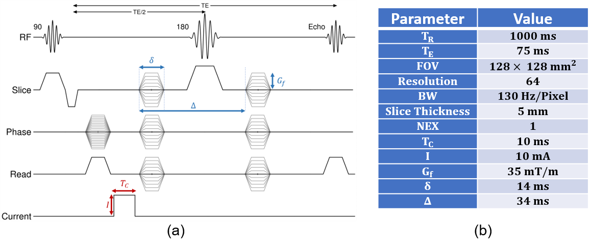
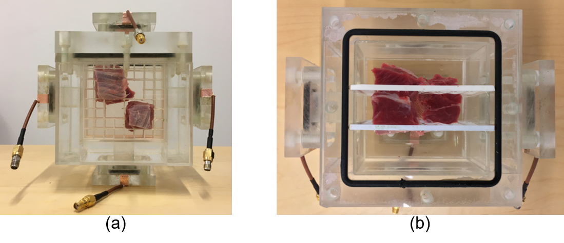
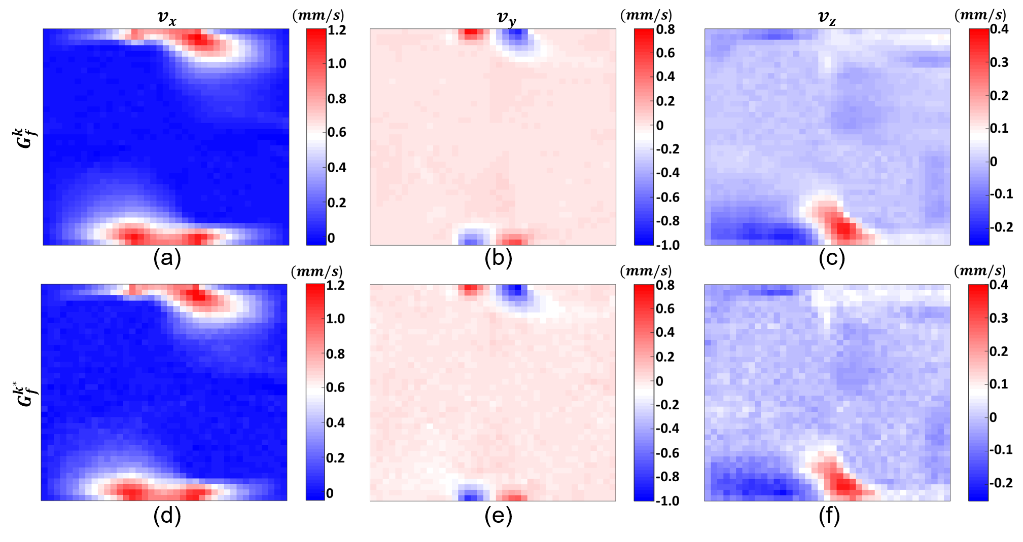
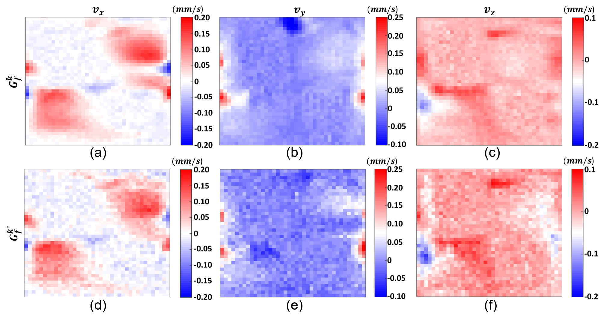
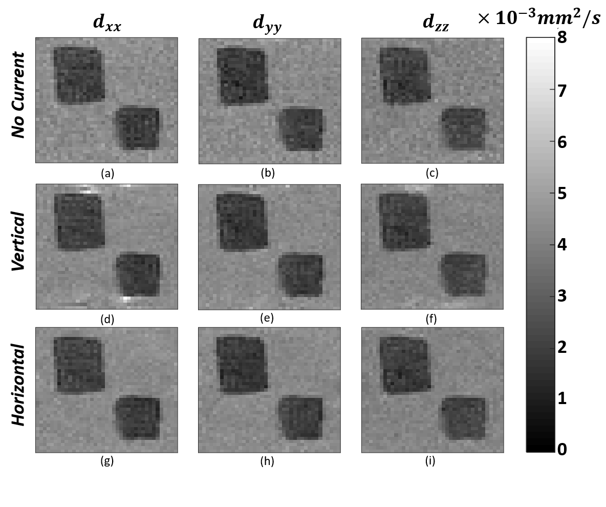
The phantom experiments are performed using a 3T MRI scanner (MAGNETOM Trio, Siemens AG, Erlangen, Germany) with the SE-based pulse sequence in Figure 1(a). The sequence parameters are given in Figure 1(b). The experimental phantom is shown in Figure 2.

The MHD flow velocity distributions obtained simultaneously with $$$\overline{\overline{D}}$$$ are shown in Figures 3 and 4 for vertical and horizontal current injection profiles, respectively. Furthermore, the corresponding $$$\overline{\overline{D}}$$$ distributions also demonstrated in Figure 5.

DISCUSSION and CONCLUSION

In Figures 3 and 4, it is seen that MHD flow velocity distributions can be obtained with the proposed flow-encoding direction set with almost the same accuracy as the results obtained using the conventional set. Similarity of the images can be observed perceptually and $$$RMSE(\%)$$$ values supports this observation.

Moreover, $$$\overline{\overline{D}}$$$ distribution is obtained using the data sets with and without current injection. The similarity between the results of the two cases shows that the current injection does not affect magnitude images as expected. Moreover, the results obtained with the current injection case have $$$\sqrt2$$$ SNR advantage since the data collection procedure is repeated twice with opposing current polarities.

One important observation is that the maximum values of the velocity distributions in Figure 3 are almost four times larger than those in Figure 4, although the injected current pulses for two cases have the same magnitude and duration. It is anticipated that this is the result of the positioning of the biological inhomogeneities. Hence, the flow dynamics in two different current injection cases get affected differently. This effect will be investigated in future studies.

References

1. Scott GC, Joy MLG, Armstrong RL, Henkelman RM. Sensitivity of Magnetic-Resonance Current-Density Imaging. J. Magn. Reson.. 1992;97(2):235-254.
2. Truong TK, Avram A, Song AW. Lorentz effect imaging of ionic currents in solution. Journal of Magnetic Resonance. 2008;191:93–99.
3. Tenforde TS. Magnetically induced electric fields and currents in the circulatory system. Progress in Biophysics and Molecular Biology. 2005;87(2-3):279–288.
4. Stäb D, Roessler J, O'Brien K, Hamilton-Craig C, Markus Barth M. ECG triggering in ultra-high field cardiovascular MRI. Tomography. 2016;2(3):167-174.
5. Balasubramanian M, Mulkern RV, Wells WMP, Sundaram P, Orbach DB. Magnetic Resonance Imaging of Ionic Currents in Solution: The Effect of Magnetohydrodynamic Flow. Magnetic Resonance in Medicine. 2015;74(4):1145–1155.
6. Minhas AS, Chauhan M, Fu F, Sadleir R. Evaluation of magnetohydrodynamic effects in magnetic resonance electrical impedance tomography at ultra‐high magnetic fields. Magnetic Resonance in Medicine. 2018;81(4):2264-2276.
7. Eroğlu HH, Sadighi M, Eyüboğlu BM. Magnetohydrodynamic flow imaging of ionic solutions using electrical current injection and MR phase measurements. Journal of Magnetic Resonance. 2019;303:128–137.
8. Benders S, Gomes BF, Carmo M, Colnago LA, Blümich B. In-situ MRI velocimetry of the magnetohydrodynamic effect in electrochemical cells. Journal of Magnetic Resonance. 2020;312:106692-106695.
9. Le Bihan D, Mangin JF, Poupon C, Clark CA, Pappata S, Molko N, Chabriat H. Diffusion Tensor Imaging: Concepts and Applications. JOURNAL OF MAGNETIC RESONANCE IMAGING. 2001 534–546.
10. Eroğlu HH, Eyüboglu BM, Göksu C. Design and implementation of a bipolar current source for MREIT applications. In: In XIII Mediterranean Conference on Medical and Biological Engineering and Computing; 2013; Seville, Spain. p. 161-164.