1256
Experimental Evaluation of Spin Echo based Magnetic Resonance Magnetohydrodynamic Flow Velocimetry1Electrical and Electronics Engineering, Middle East Technical University (METU), Ankara, Turkey, 2Danish Research Centre for Magnetic Resonance, Centre for Functional and Diagnostic Imaging and Research, Copenhagen University Hospital, Amager and Hvidovre, Denmark, 3Center for Magnetic Resonance, DTU Health Tech, Technical University of Denmark, Kgs Lyngby, Denmark
Synopsis
Magnetohydrodynamic (MHD) flow occurs due to the Lorentz force formed by the interaction between the static magnetic field of the MR scanner and the externally injected electric current. The MR based imaging of MHD flow has become a research field of interest recently. The MHD flow can be extracted from the MR phase images obtained using a pulse sequence with flow-encoding gradients. In this study, the MHD flow distributions of a simulated model and a homogeneous experimental phantom are obtained. The MHD velocity contrast images reconstructed using simulated and experimental measurements are consistent.
INTRODUCTION
Magnetic Resonance Current Density Imaging (MRCDI) is an imaging modality providing cross-sectional current density ($$$J$$$) images.1 The externally injected current pulses are applied synchronously with an MRI pulse sequence. Knowledge of $$$J$$$ is crucial in many medical applications such as tDCS and tACS.2,3 However, one important observation is that the current injection perpendicular to the static magnetic field of the MR scanner ($$$B_0$$$) causes the formation of a Lorentz force. Consequently, the Magnetohydrodynamic (MHD) flow of water molecules inside the medium takes place. Furthermore, during an electrocardiogram (ECG) triggered MRI scan, the flow of electrically conductive blood interacts with $$$B_0$$$, and induces a voltage perpendicular to $$$B_0$$$ and the flow direction. The induced voltage distorts the measured ECG.4,5 Especially, in ECG-triggered ultra-high field MRI, it is reported that the MHD effect significantly impacts the ECG signal.6Imaging the velocity distribution of the MHD flow using MRI techniques is a recent interest of research.7-11 If flow-encoding gradients are utilized, this motion is introduced as a phase term to the MR signal. MHD flow has been acquired using gradient echo (GE) and spin echo (SE) based pulse sequences and the results showed the validity of MHD flow imaging.8-10
In SE-based pulse sequences, the current is injected simultaneously with 180° RF pulse,10 or a bipolar current injection is employed in both sides of 180° RF pulse.8 The former has not been evaluated experimentally, hence the effect of the overlap is unknown while the latter suffers from the fact that bipolar current injection significantly lowers the MHD velocity and the resulting measured phase accumulation. On the other hand, the GE-based pulse sequences suffer from limited time available for the flow-encoding.9
In this study, an SE-based pulse sequence with monopolar current injection strategy is utilized to maximize the accumulated phase due to MHD flow.
METHODS
The velocity distribution of MHD flow velocity ($$$\mathbf{v}$$$) satisfies Navier–Stokes equation9:$$\rho(\frac{\partial\mathbf{v}}{\partial{t}}+\mathbf{v}\cdot\nabla\mathbf{v})=\nabla{p}+\mu\nabla^2\mathbf{v}+\mathbf{F}\quad\quad\quad\quad\quad(1)$$
where $$$\rho$$$ is the density of the fluid, $$$p$$$ is the pressure field of the domain, and $$$\mu$$$ is the dynamic viscosity. $$$\mathbf{F}$$$ is the Lorentz force can be defined as:
$$\mathbf{F}=\sigma(\mathbf{E}+\mathbf{v}\times{B_0}\mathbf{k})\times{B_0}\mathbf{k}\quad\quad\quad\quad\quad(2)$$
where $$$\sigma$$$ is the electrical conductivity and $$$\mathbf{E}$$$ is the electric field distributions of the medium.
Note that the flow-encoded phase image obtained with current injection contain the following phase components9:
$$arg(S)=\phi_0+\phi_I+\phi_{\mathbf{G_f}}+\phi_{MHD_{\mathbf{G_f}}}+\phi_{MHD_{\mathbf{G_{img}}}}\quad\quad\quad\quad\quad(3)$$
where $$$S$$$ is the complex space domain signal. $$$\mathbf{G_f}$$$ is the 3D vector which contains the intensities of flow-encoding gradients in three directions. $$$\phi_0$$$ is the systematic phase artifact, $$$\phi_I$$$ is the accumulated phase component due to the injected current. $$$\phi_{MHD_{\mathbf{G_f}}}$$$ is the phase component due to presence of the flow-encoding gradients. $$$\phi_{MHD_{\mathbf{G_f}}}$$$ and $$$\phi_{MHD_{\mathbf{G_{img}}}}$$$ are phase components created by the MHD flow. $$$\phi_{MHD_{\mathbf{G_f}}}$$$ is encoded by flow-encoding gradients and $$$\phi_{MHD_{\mathbf{G_{img}}}}$$$ is encoded by the imaging gradients.
$$$\phi_{MHD_{\mathbf{G_f}}}$$$ can be obtained as9:
$$\phi_{MHD_{\mathbf{G_f}}}=\frac{arg(S^{I_+\mathbf{G_f}_+})-arg(S^{I_-\mathbf{G_f}_+})-arg(S^{I_+\mathbf{G_f}_-})+arg(S^{I_-\mathbf{G_f}_-})}{4}\quad\quad\quad\quad\quad(4)$$
$$$S^{I_\pm\mathbf{G_f}_\pm}$$$ are space signal distributions with opposing flow-encoding gradient and current polarities.
The relation between $$$\phi_{MHD_{\mathbf{G_f}}}$$$ and the MHD flow velocity distribution can be derived as:
$$\phi_{MHD_{\mathbf{G_f}}}=-\int_{t_0}^{t_0+\delta}\gamma(\mathbf{G_f}\cdot\mathbf{v})dt+\int_{t_0+\Delta}^{t_0+\Delta+\delta}\gamma(\mathbf{G_f}\cdot\mathbf{v})dt=\gamma\delta\Delta(\mathbf{G_f}\cdot\mathbf{v})\quad\quad\quad\quad\quad(5)$$
where $$$\delta$$$ is the duration of the flow-encoding gradients and $$$\Delta$$$ is the time interval between the starting points of two consecutive flow-encoding grandients. Hence, $$$\mathbf{v}$$$ in the direction of $$$\mathbf{G_f}$$$ can be computed from $$$\phi_{MHD_{\mathbf{G_f}}}$$$.
RESULTS
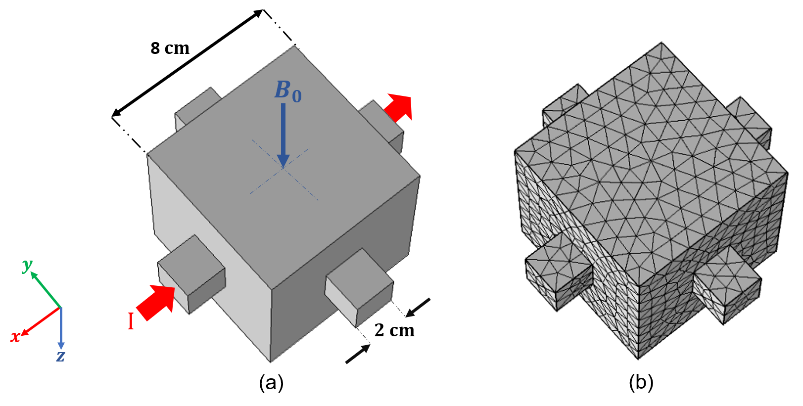
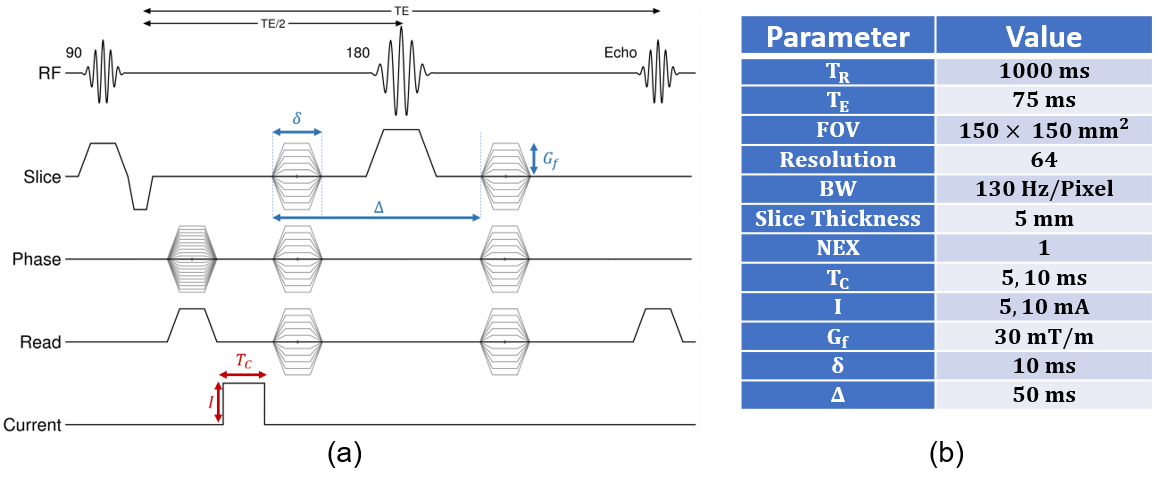
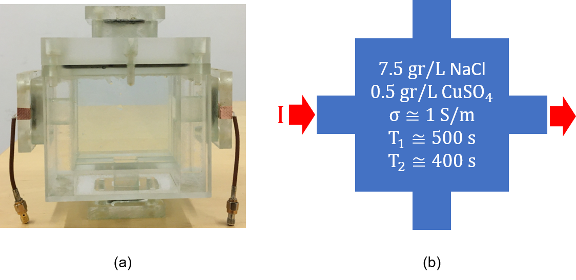
The simulation data is obtained similar to the procedure explained in10 using the Finite Element (FE) model shown in Figure 1.The phantom experiments are performed using a 3T MRI scanner (MAGNETOM Trio, Siemens AG, Erlangen, Germany) with the SE-based pulse sequence in Figure 2(a). The sequence parameters are given in Figure 2(b). The experimental phantom is shown in Figure 3.
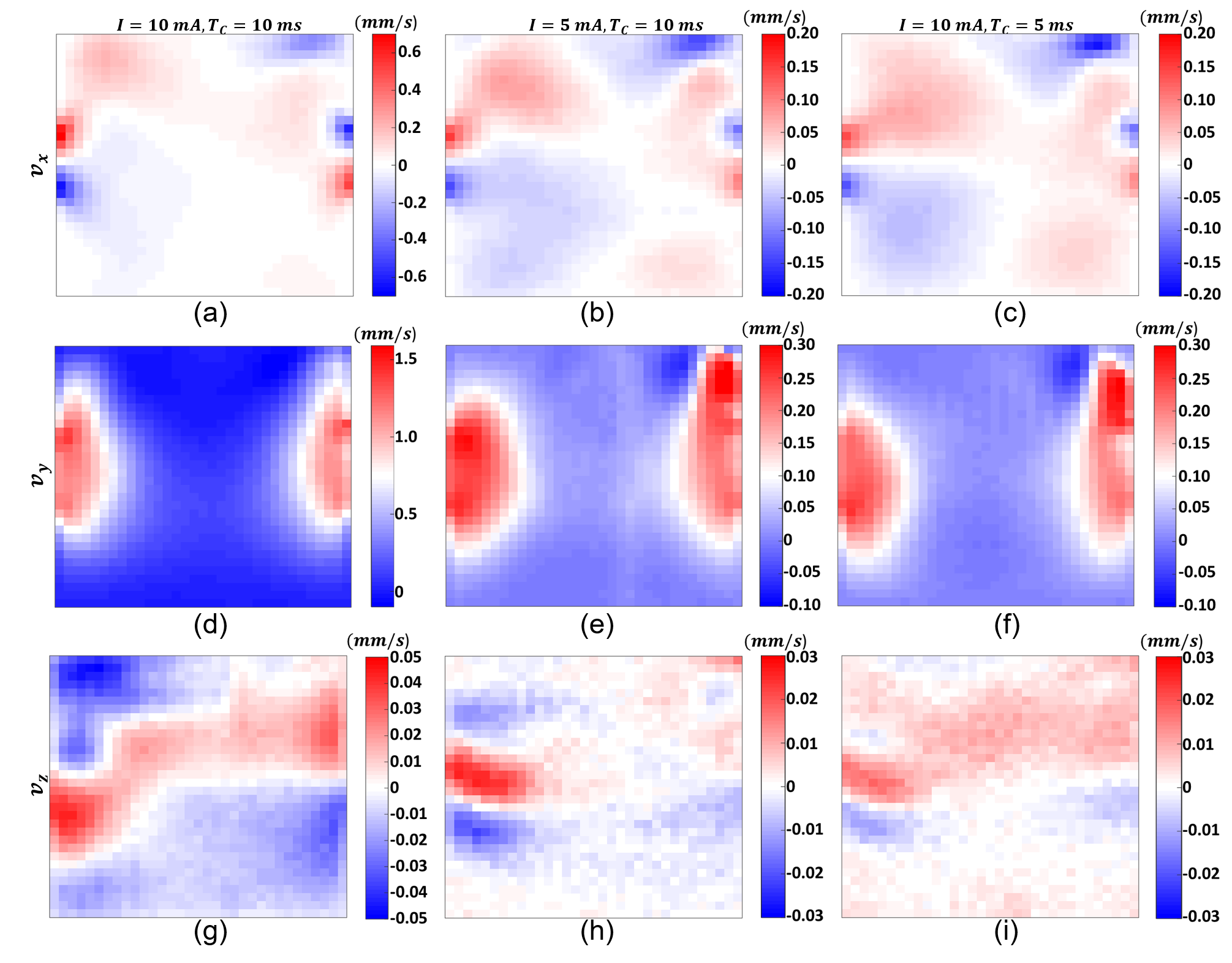
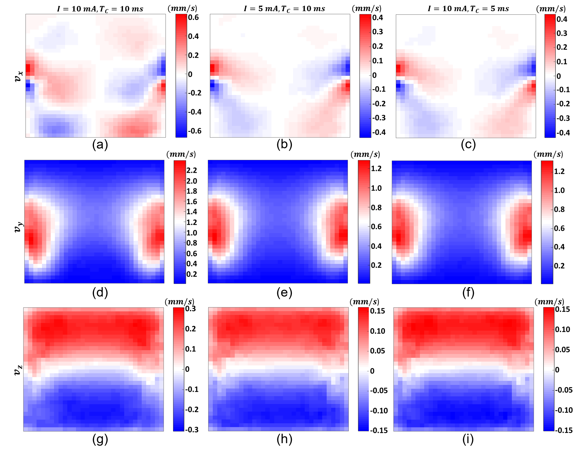
The MHD flow distributions of the FE model (Figure 1) and the experimental phantom (Figure 3) are presented in Figures 4 and 5, respectively. The experimental results are obtained using Equations 4 and 5.
DISCUSSION and CONCLUSION
As seen from Figures 4 and 5, the MHD flow velocity magnitudes are significantly larger in the y-direction than the other two orthogonal directions. This is expected since the Lorentz force is formed mainly in the y-direction by $$$B_0$$$ in the z-direction and $$$J$$$ dominant in the x-direction. Still, in some voxels around the current injection electrodes, substantial values are observed due to current dispersion. In Figure 4, distributions show a rotational motion but maximum values are relatively smaller due to the absence of the Lorentz force in this direction. In Figure 5, images demonstrate a very small range and are mostly dominated by nonideal effects.The main observation in this study is the consistency between contrasts of the simulated and the experimentally-measured MHD velocity distributions in Figures 4 and 5. However, the maximum velocity values are smaller in most of the experimentally-measured distributions. This discrepancy may arise from inadequacy in the modeling of complete flow dynamics related to the MHD flow. For instance, the Lorentz force acts on the ions in the solution, and the solvent shells are affected indirectly.8,11,13 The cause of measured values being lower than the values obtained from the simulations may be attributed to the sensitivity of MR acquisition to the movement of water molecules alone, not to the movement of ions. Nevertheless, this claim needs to be proven and will be investigated in future studies.
Acknowledgements
This work is a part of the M.Sc. thesis study of Mert Şişman. B. Murat Eyüboğlu is the thesis supervisor. Mehdi Sadighi is a graduate student under the supervision of B. Murat Eyüboğlu.
Experimental data were acquired using facilities of UMRAM (National Magnetic Resonance Research Center), Bilkent University, Ankara, Turkey.
References
1. Scott GC, Joy MLG, Armstrong RL, Henkelman RM. Sensitivity of Magnetic-Resonance Current-Density Imaging. J. Magn. Reson.. 1992;97(2):235-254.
2. Roy A, Baxter B, He B. High-definition transcranial direct current stimulation induces both acute and persistent changes in broadband cortical synchronization: a simultaneous tDCS–EEG study. IEEE Transactions on Biomedical Engineering. 2014;61(7):1967-1978.
3. Neuling T, Wagner S, Wolters CH, Zaehle T, Herrmann CS. Finite-element model predicts current density distribution for clinical applications of tDCS and tACS. Frontiers in psychiatry. 2012;3:83.
4. Tenforde TS. Magnetically induced electric fields and currents in the circulatory system. Progress in Biophysics and Molecular Biology. 2005;87(2-3):279–288.
5. Krug JW, Rose G. Magnetohydrodynamic distortions of the ECG in different MR scanner configurations. In: 2011 Computing in Cardiology; 2011. p. 769-772.
6. Stäb D, Roessler J, O'Brien K, Hamilton-Craig C, Markus Barth M. ECG triggering in ultra-high field cardiovascular MRI. Tomography. 2016;2(3):167-174.
7. Balasubramanian M, Mulkern RV, Wells WMP, Sundaram P, Orbach DB. Magnetic Resonance Imaging of Ionic Currents in Solution: The Effect of Magnetohydrodynamic Flow. Magnetic Resonance in Medicine. 2015;74(4):1145–1155.
8. Minhas AS, Chauhan M, Fu F, Sadleir R. Evaluation of magnetohydrodynamic effects in magnetic resonance electrical impedance tomography at ultra‐high magnetic fields. Magnetic Resonance in Medicine. 2018;81(4):2264-2276.
9. Eroğlu HH, Sadighi M, Eyüboğlu BM. Magnetohydrodynamic flow imaging of ionic solutions using electrical current injection and MR phase measurements. Journal of Magnetic Resonance. 2019;303:128–137.
10. Eroğlu HH, Sadighi M, Eyüboğlu BM. Magnetohydrodynamic Flow Imaging Using Spin-Echo Pulse Sequence. In: 2019 27th Signal Processing and Communications Applications Conference (SIU), IEEE; April, 2019; Sivas, Turkey. p. 1-4.
11. Benders S, Gomes BF, Carmo M, Colnago LA, Blümich B. In-situ MRI velocimetry of the magnetohydrodynamic effect in electrochemical cells. Journal of Magnetic Resonance. 2020;312:106692-106695.
12. Eroğlu HH, Eyüboglu BM, Göksu C. Design and implementation of a bipolar current source for MREIT applications. In: In XIII Mediterranean Conference on Medical and Biological Engineering and Computing; 2013; Seville, Spain. p. 161-164.
13. Luca RD. Lorentz force on sodium and chlorine ions in a salt water solution flow under a transverse magnetic field. EUROPEAN JOURNAL OF PHYSICS. 2009;30:459–466.
Figures