1255
Radiofrequency heating measurement using MR thermometry and field monitoring: methodological considerations and first in vivo results.1Paris-Saclay University, CEA, CNRS, BAOBAB, Neurospin, Gif-sur-Yvette, France, 2Skope MRT, Zurich, Switzerland, 3Paris-Saclay University, CEA, CNRS, INSERM, BioMaps, Service hospitalier Joliot, Orsay, France, 4UNIACT, Neurospin, CEA, Gif-sur-Yvette, France
Synopsis
An MR thermometry (MRT) method with field monitoring is proposed to improve the measurement of small temperature variations occurring in head MRI exams. MRT experiments were performed at 7T with concurrent radiofrequency heating and field monitoring on an agar-gel phantom and on an anaesthetized macaque. Inclusion of field fluctuations in image reconstruction showed beneficial for the measurement of small temperature rises as encountered in standard brain exams.
Introduction
With increasing magnetic field strength, the MR thermometry (MRT) PRFS (proton resonance frequency shift) method becomes more sensitive, but in addition to B0 field drift it is also more affected by external sources of frequency shift (breathing, cardiac pulsation and limb motion)1-3. NMR field sensors have shown great efficiency in monitoring and correcting in vivo for spatiotemporal field fluctuations up to the third order of the spherical harmonics decomposition4. The aim of the current study was to assess the ability of field monitoring to retrospectively correct radiofrequency (RF) induced temperature rises measured with the PRFS method at 7T to increase accuracy and precision. Preliminary measurements on an anesthetized macaque are also reported as an attempt to detect a horizontal plateau of temperature predicted by the Pennes’ model5 in the normal IEC SAR regime.Methods
MRT experiments were performed on a Magnetom 7T scanner (Siemens Healthineers, Erlangen, Germany) equipped with the Nova 1Tx-32Rx head coil (Nova Medical, Wilmington, MA, USA). A field sensors setup (Skope MRT, Zurich, Switzerland), consisting of 16 19F NMR field probes, was positioned on the receive part of the coil. Experiments were performed in vitro (agar-gel phantom) with deliberate field disturbances and in vivo on an anaesthetized macaque. In vivo scans were run twice on the same animal, months apart, to assess repeatability. Two MRT scans were acquired for each experiment: a scan without heating (approximately 0% of the maximal SAR level allowed in the IEC normal mode of operation6) and a scan at 100% SAR. For in vitro experiments, a reference temperature was measured with an optical probe at one spatial location.The MRT sequence was a single-slice 2D-GRE with TR 28 ms, TE 22/15 ms in vitro/in vivo, 3x3x5 mm3 resolution, FOV 192 mm, pixel bandwidth 2000 Hz/Px, excitation pulse flip angle 10°. An additional pulse of 3.5 ms, with 100 kHz offset was inserted in the sequence to enable RF heating while avoiding spin excitation7. The flip angle of this pulse was adjusted to reach 100% SAR. To tackle the effect of motion on the phase, three orthogonal slices were sequentially acquired and motion parameters were estimated from in vivo magnitude images8. Images were reconstructed offline using either the nominal Cartesian k-space trajectories or the actual trajectories recorded by the field sensors (FS) through an iterative conjugate gradient algorithm that included zeroth and first order field coefficients of the spherical harmonics9 (skope-i, Skope MRT, Zurich, Switzerland). Phase images were then used to compute the temperature increase ΔT=Δφ/(2πανTE), where Δφ is the phase difference, α the PRFS coefficient and ν the Larmor frequency. Despite anaesthesia, in vivo images were corrupted by motion10. Temperature was thus also computed from phase images with motion parameters regressed out11. These steps were performed both for nominal and FS-corrected images.
Results
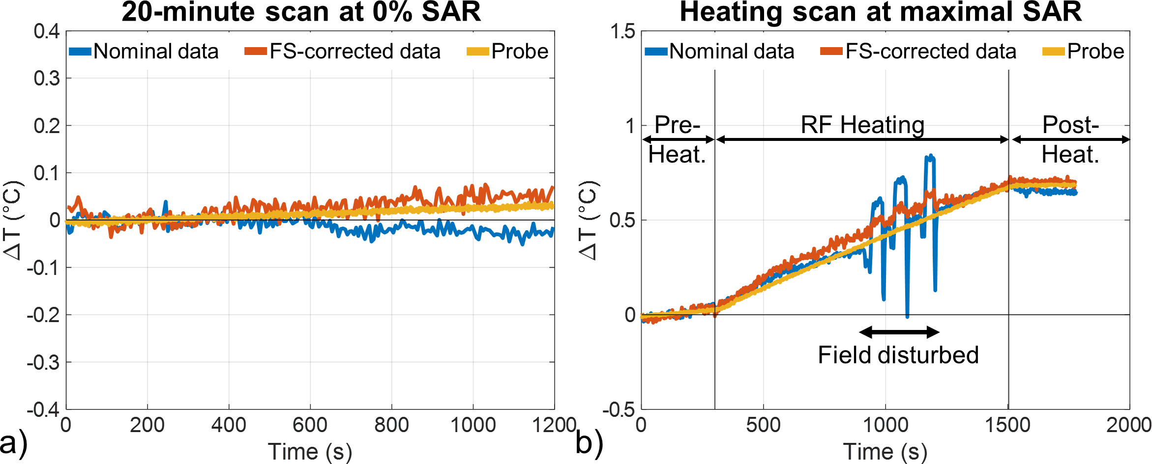
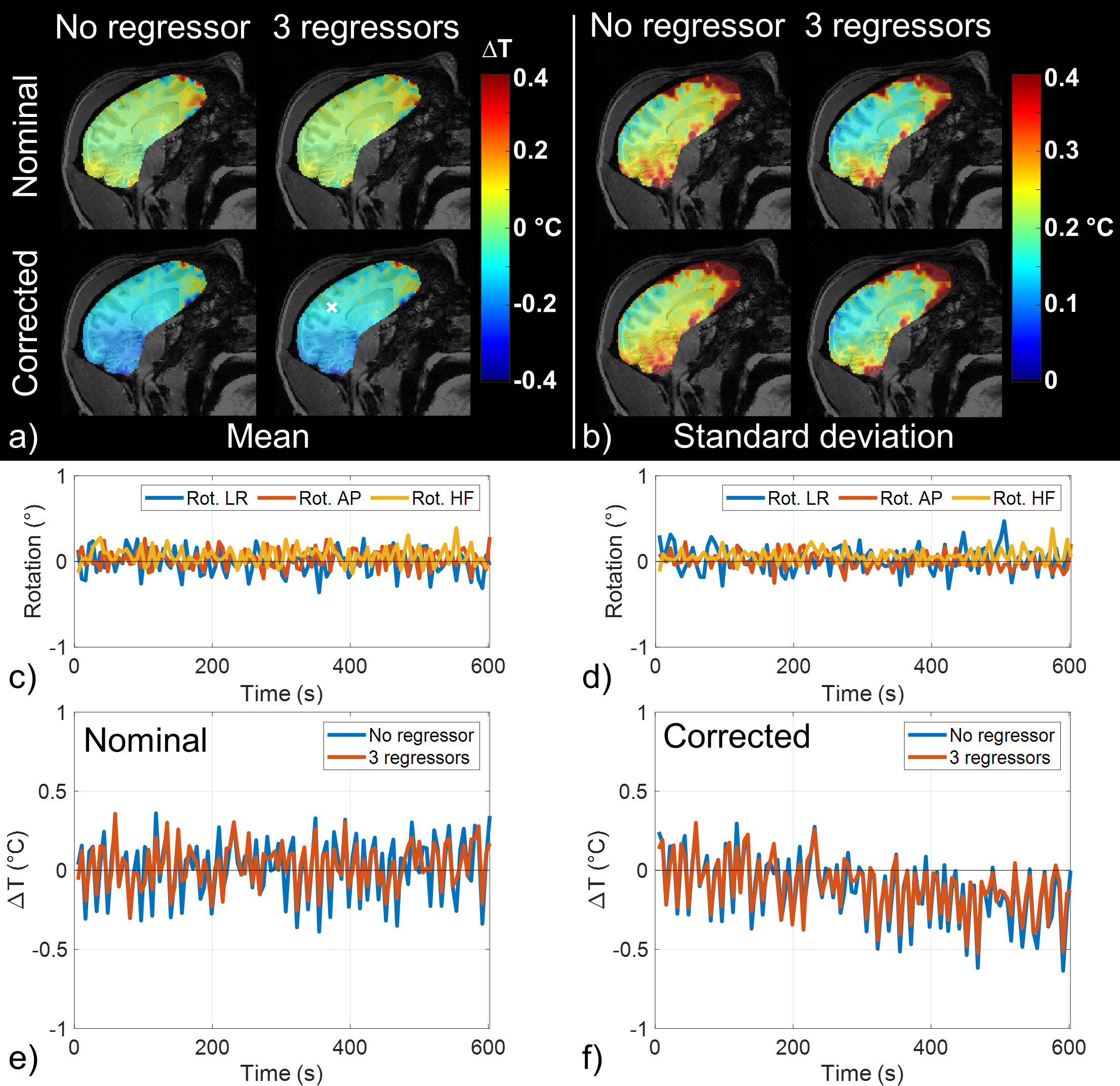
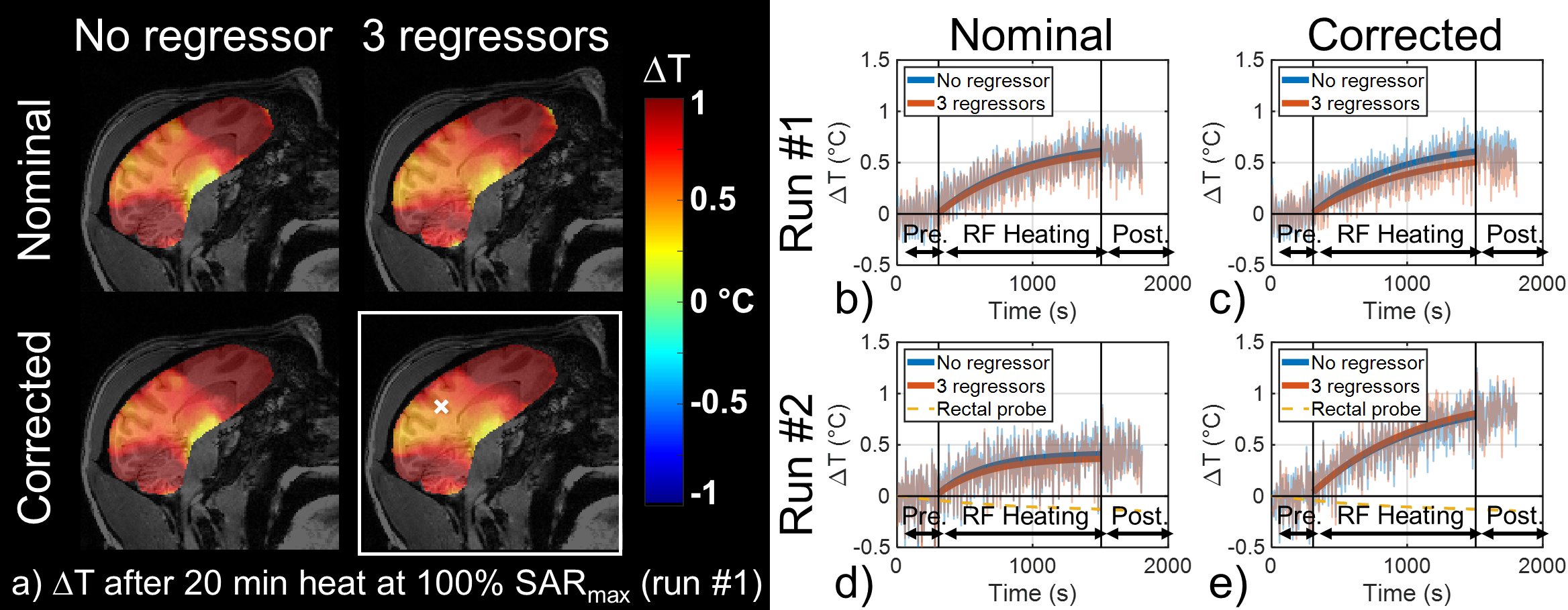
In vitro, a 20 min scan performed at 0% SAR showed that inclusion of magnetic field fluctuations in the reconstruction improved temperature measurement accuracy down to 0.02°C versus 0.03°C without correction (Figure 1a). During the heating scan (i.e. 5 min pre-heating at 0% SAR + 20 min heating at maximal SAR + 5 min post-heating at 0% SAR, Figure 1b), major field changes induced by a secondary phantom movement in the scanner tunnel were captured by the field probes and corrected to a large extent, whereas the uncorrected approach naturally failed. In vivo, during the 10 min scan performed at 0% SAR (Figure 2), there was a slow drift of the temperature computed from FS-corrected images that could not be observed on temperature computed from uncorrected images, as it was partly compensated by a slow B0 and kz drift. The standard deviation of this scan, computed from the detrended signal, was not homogeneous over the brain and reflected phase sensitivity versus motion. Inclusion of rotation regressors did not affect average temperature measurement, while it slightly reduced its standard deviation. In a voxel with low standard deviation, likely more robust to motion, a temperature fluctuation of about 0.15°C was measured. Results of the scans performed at 100% SAR (Figure 3) showed that during the heating period, temperature increased but a plateau could not be observed. A temperature increase of approximately 0.5°C (0.8°C) in the center of the macaque brain was measured after 20-minute heating for the first (second) run. With negligible heat diffusion, fitting ΔT curves obtained with FS correction during the heating period to $$$T(t)=\frac{\rho SAR}{B}(1-exp(-\frac{Bt}{\rho C_p}))$$$ returned time-constants of 12 and 13 min for runs 1 and 2 respectively, which is 3-8 times larger than expected from literature12.Discussion and conclusion
Inclusion of field fluctuations up to the first order of the spherical harmonic decomposition in image reconstruction was beneficial for the measurement of small temperature rises encountered in standard brain exams. In vivo, even if nominal images could yield comparable results to the FS-corrected ones, the field disturbance experimental data in general boosts confidence in the results obtained with field monitoring and in vivo. A horizontal temperature plateau, as predicted by Pennes bioheat model with thermal constants from literature and constant blood temperature assumption, was not observed. More work is needed to correct for motion-induced field disturbances and extract reliable temperature maps.Acknowledgements
This work received financial support from Leducq Foundation (large equipment Equipement de Recherche et Plateformes Technologiques program, NEUROVASC7T project) and from the European Union Horizon 2020 Research and Innovation program under grant agreement no. 736937 (M‐Cube project)References
1. Rieke V, Pauly KB. MR thermometry. J. Magn. Reson. Imaging 2008;27:376–390 doi: 10.1002/jmri.21265.
2. Hindman JC. Proton Resonance Shift of Water in the Gas and Liquid States. J. Chem. Phys. 1966;44:4582–4592 doi: 10.1063/1.1726676.
3. Peters RTD, Hinks RS, Henkelman RM. Ex vivo tissue-type independence in proton-resonance frequency shift MR thermometry. Magn. Reson. Med. 1998;40:454–459 doi: 10.1002/mrm.1910400316.
4. Barmet C, Zanche ND, Pruessmann KP. Spatiotemporal magnetic field monitoring for MR. Magn. Reson. Med. 2008;60:187–197 doi: 10.1002/mrm.21603.
5. Pennes HH. Analysis of Tissue and Arterial Blood Temperatures in the Resting Human Forearm. J. Appl. Physiol. 1948;1:93–122 doi: 10.1152/jappl.1948.1.2.93.
6. IEC. Medical electrical equipment-Part 2-33: Particular requirements for the basic safety and essential performance of magnetic resonance equipment for medical diagnosis. 2015;Edition 3.2.
7. Ehses P, Fidler F, Nordbeck P, et al. MRI thermometry: Fast mapping of RF-induced heating along conductive wires. Magn. Reson. Med. 2008;60:457–461 doi: 10.1002/mrm.21417.
8. Jenkinson M, Bannister P, Brady M, Smith S. Improved Optimization for the Robust and Accurate Linear Registration and Motion Correction of Brain Images. NeuroImage 2002;17:825–841 doi: 10.1006/nimg.2002.1132.
9. Wilm BJ, Barmet C, Pavan M, Pruessmann KP. Higher order reconstruction for MRI in the presence of spatiotemporal field perturbations. Magn. Reson. Med. 2011;65:1690–1701 doi: 10.1002/mrm.22767.
10. Liu J, de Zwart JA, van Gelderen P, Murphy-Boesch J, Duyn JH. Effect of head motion on MRI B0 field distribution: Liu et al. Magn. Reson. Med. 2018;80:2538–2548 doi: 10.1002/mrm.27339.
11. Hutton C, Andersson J, Deichmann R, Weiskopf N. Phase informed model for motion and susceptibility: Phase Informed Model for Motion and Susceptibility. Hum. Brain Mapp. 2013;34:3086–3100 doi: 10.1002/hbm.22126.
12. Collins CM, Liu W, Wang J, et al. Temperature and SAR calculations for a human head within volume and surface coils at 64 and 300 MHz. Journal of Magnetic Resonance Imaging 2004;19:650–656 doi: 10.1002/jmri.20041.
Figures