1239
Multi-Physics Multi-Contrast Magnetic Resonance Imaging1Electrical and Electronics Eng., Middle East Technical University (METU), Ankara, Turkey
Synopsis
In this study, a Diffusion-Weighted (DW) Spin Echo (SE) based pulse sequence with current injection is proposed to combine data acquisitions of the Diffusion Tensor ($$$\overline{\overline{D}}$$$), current-induced magnetic flux density $$$B_z$$$ and the magnetohydrodynamic (MHD) flow imaging. The current density distribution ($$$\overline{J}$$$) can be estimated from the measured $$$B_z$$$ using the MRCDI method and the conductivity tensor can be reconstructed from the acquired $$$\overline{\overline{D}}$$$ and the estimated $$$\overline{J}$$$ using the DT-MREIT method. The acquired results of an experimental phantom with anisotropic diffusion using DW-SE pulse sequence shows that the proposed method could provide multi-contrast imaging based on multiple physical properties.
INTRODUCTION
The electrical properties of biological tissues determine the current flow pathways through tissues and vary depending on the tissues’ anatomical structure or physiological state.1-3 The knowledge of the current-induced $$$B_z$$$ and $$$\overline{J}$$$ of the impressed currents in the mA range is essential in many medical applications to optimize and plan treatments like tDCS, tACS, or deep brain stimulation.4-10 The MRCDI modality provides cross-sectional $$$\overline{J}$$$ distributions of externally injected currents in synchrony with an MRI pulse sequence.11 Besides, $$$B_z$$$ and $$$\overline{J}$$$ are key information to reconstruct the conductivity distributions of biological tissues using magnetic resonance electrical impedance tomography (MREIT)12 and diffusion tensor-MREIT.13 DT-MREIT is based on the linear relationship between the conductivity tensor ($$$\overline{\overline{C}}$$$) and $$$\overline{\overline{D}}$$$ in a porous medium: $$\overline{\overline{C}}=\eta{\overline{\overline{D}}}\qquad[1]$$ $$$\eta$$$ is the extra-cellular conductivity and diffusivity ratio (ECDR), which can be calculated from the acquired $$$\overline{J}$$$ and $$$\overline{\overline{D}}$$$. In DT-MREIT, $$$\overline{\overline{D}}$$$ and $$$\overline{J}$$$ data are acquired separately from DTI and MRCDI methods. This study aims to combine DTI and MRCDI data acquisitions to provide $$$\overline{\overline{D}}$$$, $$$B_z$$$, $$$\overline{J}$$$ and consequently $$$\overline{\overline{C}}$$$ simultaneously. Furthermore, due to the interaction between the static magnetic field of the MR scanner ($$$B_0$$$) and the externally injected current magnetohydrodynamic (MHD) flow occurs, which is encoded into the MR signal in the presence of diffusion-encoding gradients of DTI. In this study, a diffusion-weighted (DW) Spin-Echo (ES) pulse sequence with simultaneous current injection is developed for multi-contrast imaging.METHODS
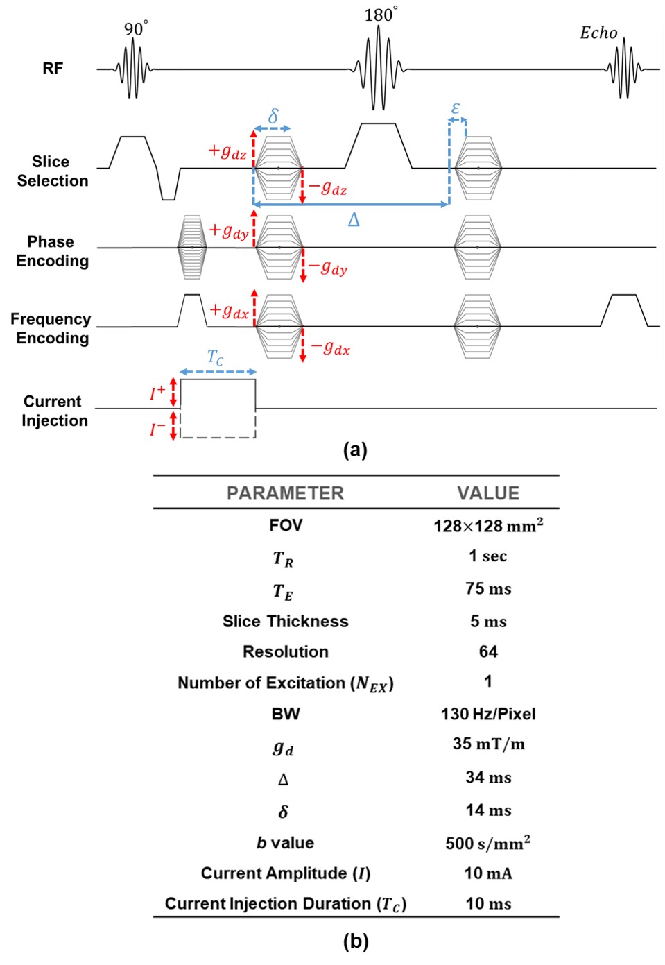
DW-SE pulse sequence can provide high-quality, high-resolution DW images with minimal artifacts14 without the need for post-processing corrections required for DW-EPI pulse sequence. The DW-SE pulse sequence yielding multi-contrast images is shown in Fig.1(a).The MR signal of the DW-SE pulse sequence can be expressed as:$$ S_k=S_0\:e^{-b{\overline{g}}_{d_{k}}\overline{\overline{D}}{\overline{g}}_{d_{k}}^T}\:e^{-j(\phi_I+\phi_{g_d}+\phi_{{MHD}_{g_d}}+\phi_{{MHD}_{G_R}})}\qquad{\text{for}\qquad{k=1...N_D}}\qquad[2]$$ where, $$$S_k$$$ is the MR signal obtained by applying the diffusion-encoding gradient $$${\overline{g}_{d_k}}={g}_{d_k}[u_k\:v_k\:w_k]$$$.$$$u$$$, $$$v$$$ and $$$w$$$ are the direction cosines of the diffusion gradient vector. $$$\phi_I$$$ is the accumulated phase due to the current-induced $$$B_z$$$. $$$\phi_{g_d}$$$ is the phase component due to the diffusion-encoding gradient application. $$$\phi_{MHD_{g_d}}$$$ and $$$\phi_{MHD_{G_R}}$$$ are the phase components created due to the MHD flow and encoded to the MR signal by diffusion-encoding and imaging gradients, respectively. $$$N_D$$$ is the total number of diffusion-encoding directions. $$$b$$$ value controls the degree of diffusion weighting and is defined as:$$ b=\gamma^2g_d^2\left(\delta^2(\Delta-\frac{\delta}{3})+\frac{\varepsilon^3}{30}-\frac{\delta\varepsilon^2}{6}\right)\qquad[3]$$ To successfully reconstruct $$$\overline{\overline{D}}$$$, $$$B_z$$$ and MHD flow from the MR signal in Eq.2, the data is acquired two times with $$$I^{\pm}$$$ in $$$k=6$$$ diffusion-encoding directions as:$$ [u_k\:v_k\:w_k]=[\frac{1}{\sqrt2}\:0\:\frac{1}{\sqrt2}],[\frac{-1}{\sqrt2}\:0\:\frac{1}{\sqrt2}],[\frac{1}{\sqrt2}\:\frac{1}{\sqrt2}\:0],[\frac{1}{\sqrt2}\:\frac{-1}{\sqrt2}\:0],[0\:\frac{1}{\sqrt2}\:\frac{1}{\sqrt2}],[0\:\frac{1}{\sqrt2}\:\frac{-1}{\sqrt2}]\qquad[4]$$ Furthermore, two sets of data are acquired with $$$I^{\pm}$$$ and without applying diffusion-encoding gradients to be used in the reconstruction of $$$\overline{\overline{D}}$$$ and $$$B_z$$$. $$$\overline{\overline{D}}$$$ at each voxel can be represented as a 3x3 matrix and can be reconstructed from the MR magnitude images by solving the following system of equations:$$ \overline{\overline{G}}\:\overline{d}=\overline{s}\quad\equiv\quad\begin{bmatrix}u_1^2&v_1^2&w_1^2&2u_1v_1&2u_1w_1& 2v_1w_1\\u_2^2& v_2^2&w_2^2&2u_2v_2&2u_2w_2&2v_2w_2\\ \vdots&\vdots&\vdots&\vdots&\vdots&\vdots\\u_6^2&v_6^2&w_6^2 &2u_6v_6&2u_6w_6&2v_6w_6\end{bmatrix}\begin{bmatrix}d_{xx}\\d_{yy}\\d_{zz}\\d_{xy}\\d_{xz}\\d_{yz}\end{bmatrix}=\frac{1}{b}\begin{bmatrix}\ln(\frac{S_0}{\mid{S_1}\mid})\\{\ln(\frac{S_0}{\mid{S_2}\mid})}\\{\ln(\frac{S_0}{\mid{S_3}\mid})}\\{\ln(\frac{S_0}{\mid{S_4}\mid})}\\{\ln(\frac{S_0}{\mid{S_5}\mid})}\\{\ln(\frac{S_0}{\mid{S_6}\mid})}\end{bmatrix}\qquad[5]$$ MHD flow distribution can be reconstructed as15,16:$$ \phi_{MHD_{g_d}}=\frac{\arg\left({S_k}^{I^+,\:{\overline{g}_d}^+}\right)-\arg\left({S_k}^{I^-,\:{\overline{g}_d}^+}\right)-\arg\left({S_k}^{I^+,\:{\overline{g}_d}^-}\right)+\arg\left({S_k}^{I^-,\:{\overline{g}_d}^-}\right)}{4}\qquad[6]$$ $$${S_k}^{I^{\pm},\:{\overline{g}_d}^{\pm}}$$$ denotes the signal obtained using opposing polarities of $$$I$$$ and $$$\overline{g}_d$$$. $$$B_z$$$ distribution can be reconstructed from the phase images of the measurements with $$$I^{\pm}$$$ but without flow encoding gradients as:$$ B_z=\frac{\arg{\left(S^{I^+}\right)}-\left(S^{I^+}\right)}{2\gamma{T_C}}\qquad[7]$$ $$$\gamma$$$ is the gyromagnetic constant of the hydrogen proton. The projected current density $$$\overline{J}_p $$$ can be estimated from the measured $$$B_z$$$ as:17 $$ \overline{J}_p=\overline{J}_0+\frac{1}{\mu_0}\left(\frac{\partial(B_z-B_z^0)}{\partial{y}}\quad-\frac{\partial(B_z-B_z^0)}{\partial{x}}\quad0\right)\qquad[8]$$ Finally, $$$\overline{\overline{C}}$$$ can be reconstructed from $$$\overline{\overline{D}}$$$ and $$$\overline{J}_p$$$ using the DT-MREIT method.18,19
RESULTS
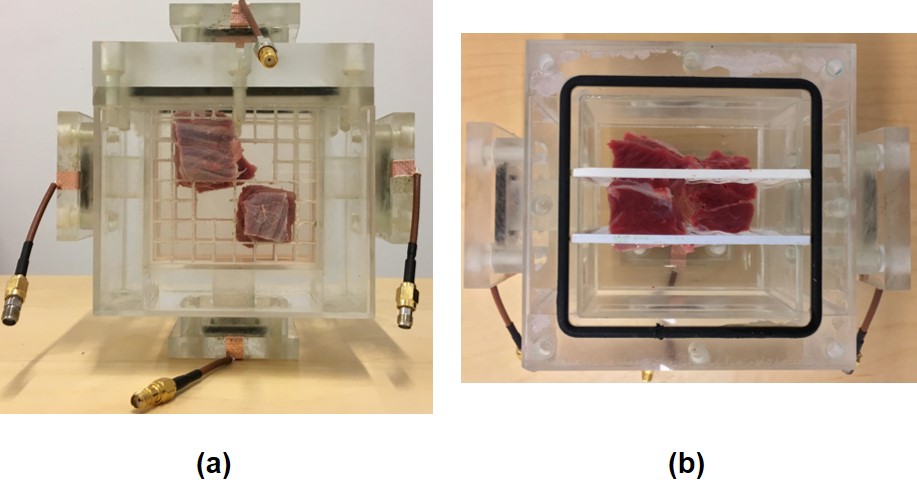
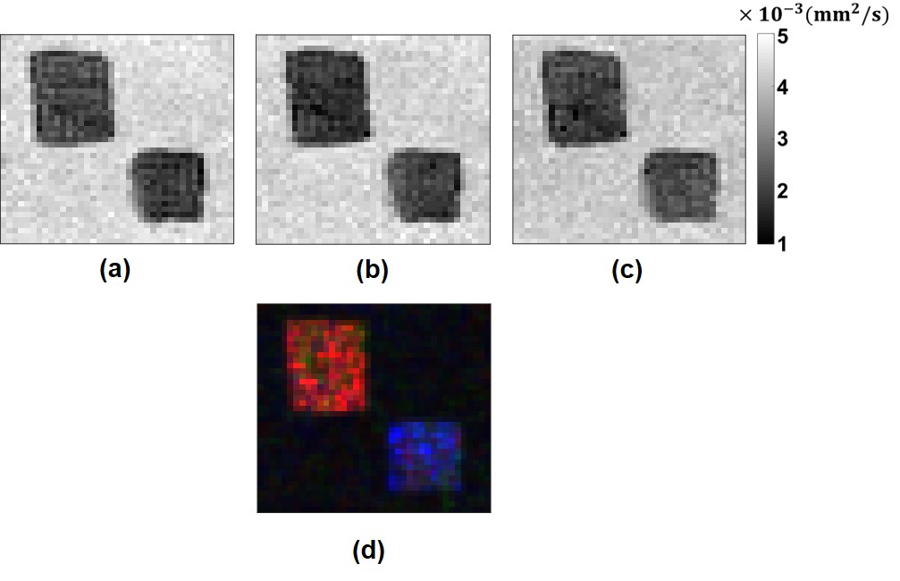
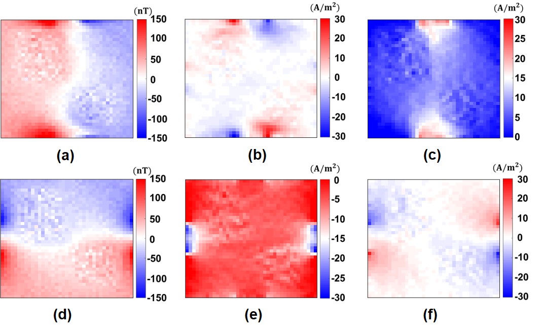
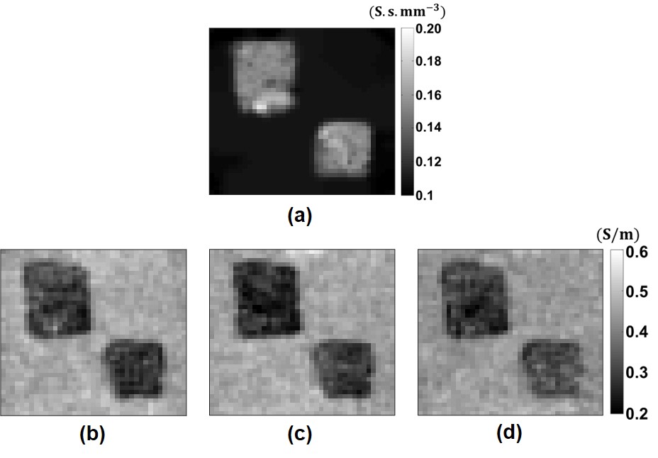
A 3T clinical MRI scanner (MAGNETOM Trio, SIEMENS) with the maximum gradient strength of 45 mT/m is used. DW-SE pulse sequence in Fig.1(a) is used with parameters in Fig.1(b). The experimental phantom is shown in Fig.2.The reconstructed $$$\overline{\overline{D}}$$$ distribution of the experimental phantom from the acquired DW images by DW-SE pulse sequence is shown in Fig.3. $$$\overline{\overline{D}}$$$ is reconstructed from the averaging of two sets of DW images obtained in six diffusion directions with opposite current polarities and two T2-weighted images with $$$I^{\pm}$$$ but without flow encoding gradients (fourteen in total). The measured $$$B_z$$$ and the estimated $$$\overline{J}_p $$$ distributions are shown in Fig.4(a) and (b), respectively. The reconstructed $$$\eta$$$ and $$$\overline{\overline{C}}$$$ distributions are shown in Fig.5(a) and (b-c), respectively.
DISCUSSION & CONCLUSION
The results of the reconstructed $$$\overline{\overline{D}}$$$, $$$B_z$$$, $$$\overline{J}_p$$$ and $$$\overline{\overline{C}}$$$ show that the proposed DW-SE pulse sequence with current injection (Fig.1) could provide multi-contrast images of the experimental phantom simultaneously. The results related to the MHD flow can be extracted from the MR phase images of the DW-SE pulse sequence, as shown in Eq.6. However, the theory behind and the reconstructed MHD flow distributions are the subject of another study and are not reported here. The mean values of the reconstructed $$$\overline{\overline{D}}$$$ for the left and right inhomogeneities are given in Fig.3, which shows the amount of anisotropy in the muscle pieces. The colored FA map shows that the diffusion in the left and right inhomogeneities are mainly in the x- and z- directions, respectively. The $$$\eta$$$ and the $$$\overline{\overline{C}}$$$ distributions are reconstructed using the $$$\overline{\overline{D}}$$$ distribution in Fig.3 and the estimated $$$\overline{J}_p$$$ in Fig.4 using the double-current DT-MREIT method.18,19 The mean values of the reconstructed $$$\overline{\overline{C}}$$$ for the left and right inhomogeneities are given in Fig.5 and show an anisotropy similar to the reconstructed $$$\overline{\overline{D}}$$$ which is expected since the $$$\overline{\overline{C}}$$$ and $$$\overline{\overline{D}}$$$ share eigenvectors in a porous medium as given in Eq.1.Acknowledgements
This work is a part of the Ph.D. thesis study of Mehdi Sadighi. B. Murat Eyüboğlu is the thesis supervisor. Mert Şişman is a graduate student under the supervision of B. Murat Eyüboğlu.
Experimental data were acquired using the facilities of UMRAM (National Magnetic Resonance Research Center), Bilkent University, Ankara, Turkey.
References
1. Surowiec AJ, Stuchly SS, Barr JR, Swarup A. Dielectric properties of breast carcinoma and the surrounding tissues. IEEE Tran Biomed Eng. 1988;35(4):257-263.
2. Joines WT, Zhang, Li C, Jirtle RL. The measured electrical properties of normal and malignant human tissues from 50 to 900 MHz. J Med Phys. 1994;21(4):547-550.
3. Miklavčič D, Pavšelj N, Hart FX. Electric Properties of Tissues. In: Wiley Encyclopedia of Biomedical Engineering. American Cancer Society; 2006.
4. Hömmen P, Storm JH, Höfner N, Körber R. Demonstration of full tensor current density imaging using ultra-low field MRI. Magn Reson Imaging. 2019;60:137-144.
5. Roy A, Baxter B, He B. High-definition transcranial direct current stimulation induces both acute and persistent changes in broadband cortical synchronization: a simultaneous tDCS–EEG study. IEEE Trans Biomed Eng. 2014;61(7):1967-1978.
6. Miranda PC, Lomarev M, Hallett M. Modeling the current distribution during transcranial direct current stimulation. Clin Neurophysiol. 2006;117(7):1623-1629.
7. Wagner T, Fregni F, Fecteau S, Grodzinsky A, Zahn M, Pascual-Leone A. Transcranial direct current stimulation: a computer-based human model study. Neuroimage. 2007;35(3):1113-1124.
8. Neuling T, Wagner S, Wolters CH, Zaehle T, Herrmann CS. Finite-element model predicts current density distribution for clinical applications of tDCS and tACS. Frontiers in psychiatry. 2012;3(83):1-10.
9. Limousin P, Krack P, Pollak P, Benazzouz A, Ardouin C, Hoffmann D, Benabid AL. Electrical stimulation of the subthalamic nucleus in advanced Parkinson's disease. N Engl J Med. 1998;339(16):1105-1111.
10. Johnson MD, Lim HH, Netoff TI, Connolly AT, Johnson N, Roy A, Holt A, Lim KO, Carey JR, Vitek JL, et al. Neuromodulation for brain disorders: challenges and opportunities. IEEE Trans Biomed Eng. 2013;60(3):610-624.
11. Scott GC, Joy MLG, Armstrong RL, Henkelman RM. Sensitivity of Magnetic-Resonance Current-Density Imaging. J Magn Reson 1992;97(2):235-254.
12. Eyüboğlu BM. Magnetic resonance electrical impedance tomography. Wiley Encyclopedia of Biomedical Engineering. 2006;4: 2154–2162.
13. Kwon OI, Jeong WC, Sajib SZ, Kim HJ, Woo EJ. Anisotropic conductivity tensor imaging in MREIT using directional diffusion rate of water molecules. Phys Med Biol. 2014;59(12):2955-2974.
14. de Crespigny AJ, Marks MP, Enzmann DR, Moseley ME. Navigated diffusion imaging of normal and ischemic human brain. Magn Reson Med. 1995;33(5):720-728.
15. Eroğlu HH, Sadighi M, Eyüboğlu BM. Magnetohydrodynamic flow imaging of ionic solutions using electrical current injection and MR phase measurements. J. Magn. Reson. 2019;303:128–137.
16. Eroğlu HH, Sadighi M, Eyüboğlu BM. Magnetohydrodynamic Flow Imaging Using Spin-Echo Pulse Sequence. 27th Signal Processing and Communications Applications Conference (SIU); 2019. p.1-4.
17. Park C, Lee BI, Kwon OI. Analysis of recoverable current from one component of magnetic flux density in MREIT and MRCDI. Phys Med Biol. 2007;52(11):3001-3013.
18. Sadighi M, Şişman M, Açıkgöz BC, Eyüboğlu BM. Single Current Diffusion Tensor Magnetic Resonance Electrical Impedance Tomography: A Simulation Study at the 2020 ISMRM & SMRT Virtual Conference & Exhibition, 2020. #3233.
19. Sadighi M, Şişman M, Açıkgöz BC, Eyüboğlu BM. Experimental Realization of Single Current Diffusion Tensor Magnetic Resonance Electrical Impedance Tomography at the 2020 ISMRM & SMRT Virtual Conference & Exhibition, 2020. #0179.
Figures