1188
Automatic determination of the regularization weighting for wavelet-based compressed sensing MRI reconstructions1Centre for Functional and Metabolic Mapping, Robarts Research Institute, Western University, London, ON, Canada, 2Department of Medical Biophysics, Schulich School of Medicine and Dentistry, Western University, London, ON, Canada
Synopsis
Most compressed sensing reconstruction procedures have relied on user-defined tuning and/or multiple comparisons to the fully sampled data to demonstrate both the feasibility of compressed sensing reconstructions as the appropriate selection of the regularization weighting. Obviously, this is a time-consuming procedure which could be avoided if we had a method that provides the regularization weighting in an automatic, non-iterative, prospective, and fast manner. Here, we present such method that could significantly accelerate research that is based on compressed sensing and improve its clinical translatability when the sparsifying domain is based on the wavelet transform.
Purpose
Most commonly used strategies to determine the regularization weighting, $$$\lambda$$$, in the field of compressed sensing1 (CS) MRI reconstructions2–10,$$\hat{x}=\textrm{argmin}_x \ \ \|Ax-y\|_2^2 +\lambda\|\Psi x\|_1 \ \ \ \textrm{(1)}$$
rely on the evaluation of multiple reconstructions in order to determine $$$\lambda$$$. An incorrect $$$\lambda$$$ can easily generate artifacts, smoothing, and loss in both structural information as in noise suppression. Here, we present an approach that automatically and rapidly determines the regularization weighting for wavelet-based compressed sensing reconstructions. This technique determines prospectively level-specific regularization weighting factors in the wavelet transform from the inverse Fourier transform of the zero-filled $$$k$$$-space.
Theory
Our approach to determine the automatic regularization weighting, from Eq. (3), can be described in two main steps.1- Estimation of the maximum decomposition level for the wavelet transform:
We measure sparsity per decomposition level by means of the Gini index11 and determine the maximum decomposition level by increasing the decomposition level until the Gini index for the next level decreases.
2- Determination of level-dependent regularization weighting:
We define a level-dependent regularization weighting as the boundary between the body and the tails of each wavelet coefficients’ histogram using a $$$k$$$-means algorithm ($$$k$$$=2). The feature for allocation is the frequency from each histogram.
Without loss of generality, the typically scalar value of $$$\lambda$$$ in Eq. (1), can also be a diagonal matrix. Thus, the soft-thresholding function, which is the proximal operator12,13 of the regularizer in Eq. (1), $$$ \lambda \| \Psi x \|_1 $$$, can be performed level-wise.
Methods
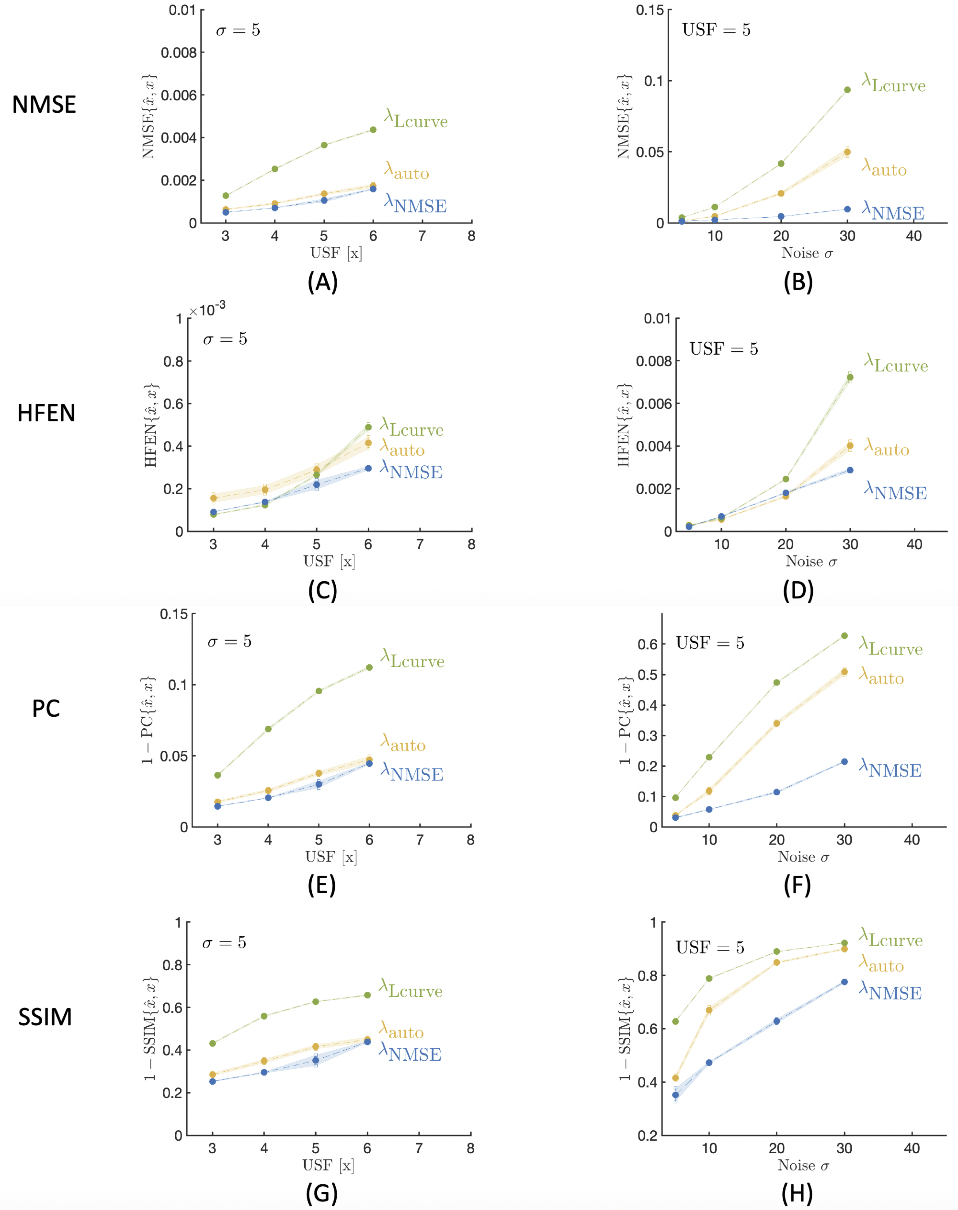
In vivo and simulated data were retrospectively under-sampled using a Poisson distribution. Additionally, we sample 24 calibration lines in order to estimate coil sensitivities with ESPIRIT14. For complex reconstructions we solve Eq. (1) with our own implementation of FISTA15. For the sparsifying domain, $$$\Psi$$$, we use the 4th level Daubechies mother wavelet. Here, we compare three methods to obtain $$$\lambda $$$: 1) our approach, $$$\lambda_{\textrm{auto}}$$$ , 2) the L-curve16, $$$\lambda_{\textrm{Lcurve}}$$$, and 3) the minimum normalized mean squared error (NMSE)2,4,8, $$$\lambda_{\textrm{NMSE}}$$$. To obtain either $$$ \lambda_{\textrm{Lcurve}}$$$ or $$$\lambda_{\textrm{NMSE}}$$$, we evaluate a range of regularization weightings to select the one that best fits to each criterion, respectively. We include the same analysis for different decomposition levels of the wavelet transform to show its effect in the reconstruction for all methods.Then, we used the simulations to analyze the reconstruction performance for different noise levels (from $$$\sigma$$$=5 to $$$\sigma$$$=30 as standard deviation of the noise) and for different under-sampling factors (from 3x to 6x) with the objective of studying the impact of these variables and to compare our approach to the results from selecting the regularization weighting using L-curve and NMSE. For the evaluation, we use multiple reconstruction quality indices: the normalized mean squared error (NMSE), the Pearson’s correlation coefficient (PC), the high frequency error norm (HFEN) and the structural similarity index (SSIM). We repeat each combination of under-sampling and noise level ten times to compute mean and standard deviation from the different reconstruction quality indices.
Results
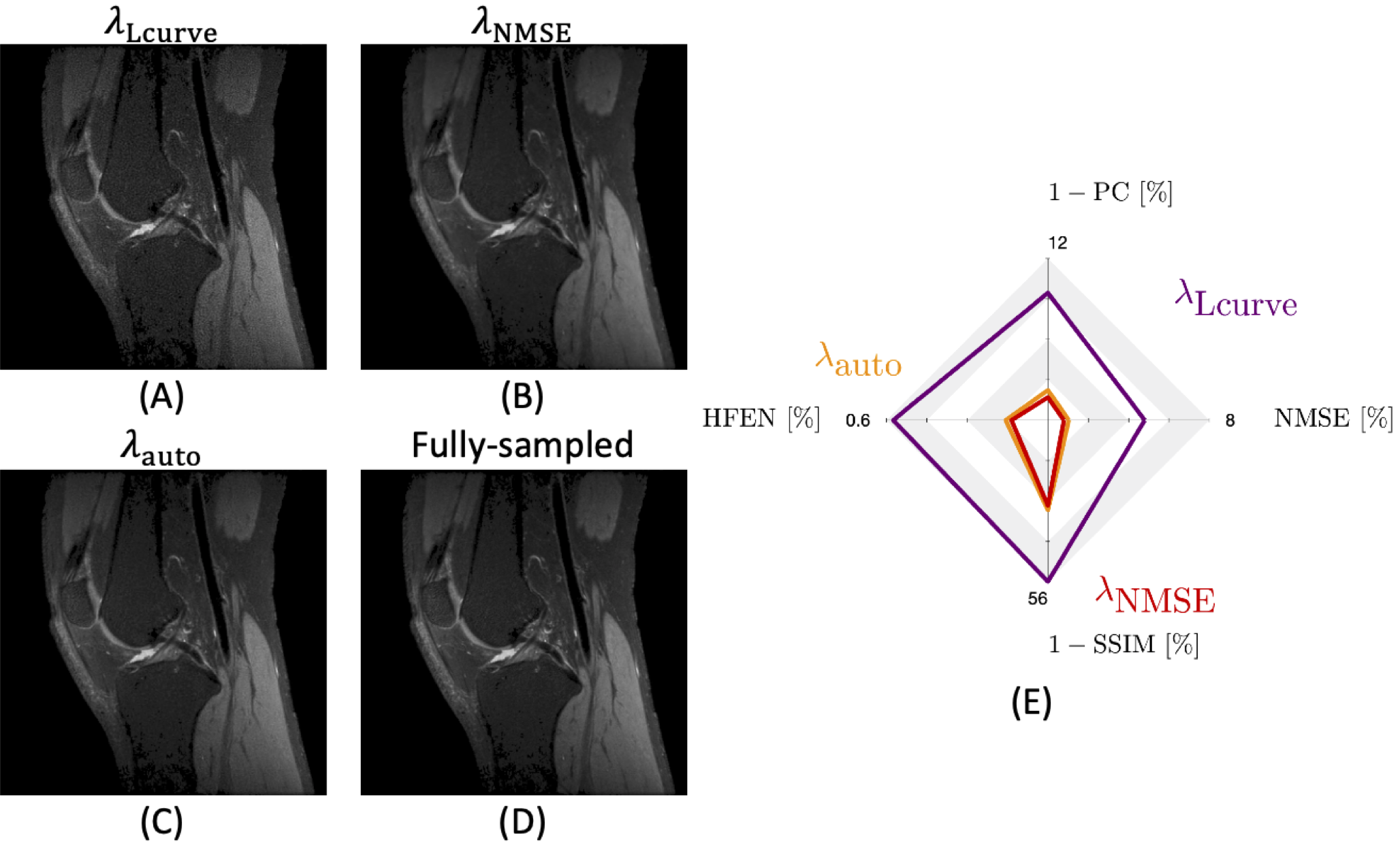
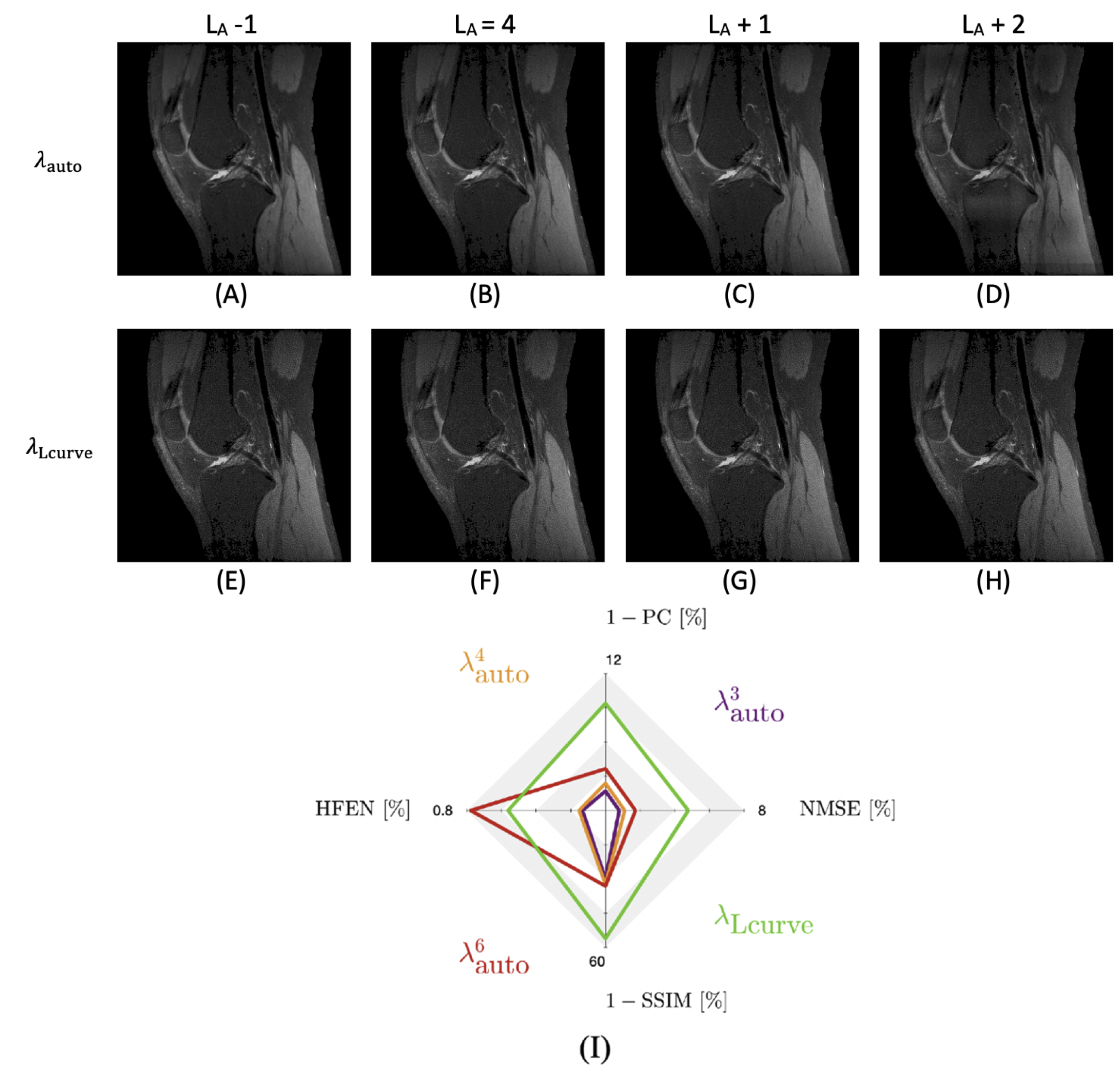
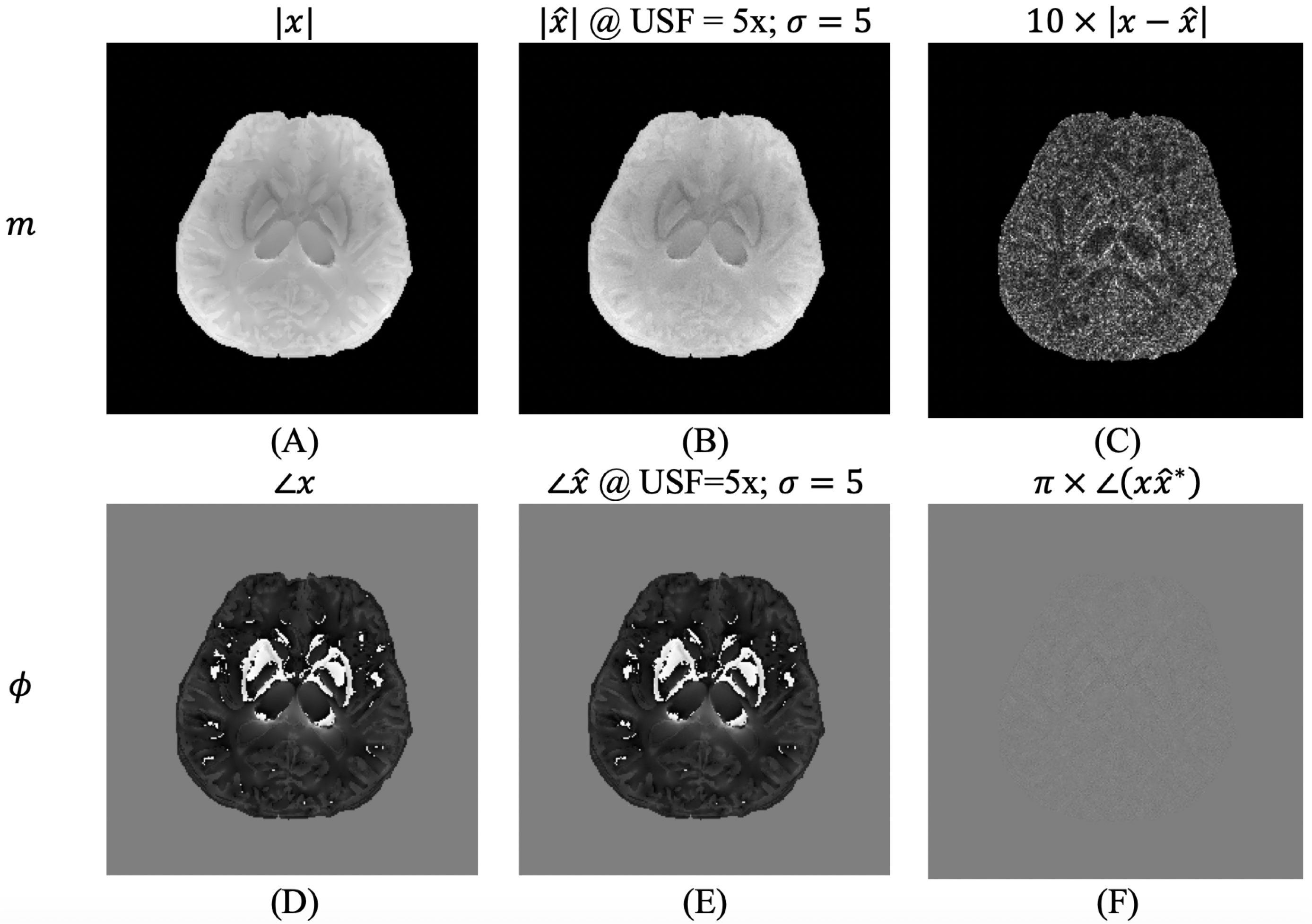
Figures 1 shows that our proposed approach, $$$\lambda_{\textrm{auto}}$$$, obtains a regularization weighting which provides improved reconstruction quality as the result obtained using $$$\lambda_{\textrm{Lcurve}}$$$ and comparable quality to $$$\lambda_{\textrm{NMSE}}$$$. Figure 2 shows the effect of the decomposition level for our approach and for the L-curve strategy. Panel (D) shows that increasing the decomposition level past the level determined by step 1 of our approach may lead to artifacts. Meanwhile, $$$\lambda_{\textrm{Lcurve}}$$$ is invariant to the decomposition level. The quantitative analysis on panel (I) shows that the reconstruction quality obtained with our approach, given an appropriate decomposition level, has better reconstruction quality than the one obtained by the L-curve. The best reconstruction performance is obtained by using our approach with three decomposition levels; however, our automatic approach has the second-best reconstruction performance and differences are quite minor from a qualitative point of view. Figure 3 shows the reconstruction performance obtained from $$$\lambda_{\textrm{auto}}$$$, $$$\lambda_{\textrm{NMSE}}$$$ and $$$\lambda_{\textrm{Lcurve}}$$$ as a function of the under-sampling pattern (USF) and the noise level ($$$\sigma$$$). The different reconstruction quality indices show the similarity and differences between the results from our approach and the results from either L-curve or NMSE strategies. Figure 4 shows that magnitude and phase images, obtained by our approach with one fifth of the data and $$$\sigma=5$$$ (SNR = 20), preserve most of the structural features of interest; however, it may be necessary to decrease the under-sampling factor when the noise level increases or to improve image reconstruction quality.In summary, our proposal, $$$\lambda_{\textrm{auto}}$$$, provides improved reconstructed image quality to that obtained by $$$\lambda_{\textrm{Lcurve}}$$$ regardless of under-sampling or SNR and comparable quality to $$$\lambda_{\textrm{NMSE}}$$$ at high SNR. Our approach reduces reconstruction time by avoiding unnecessary reconstructions to determine the “ideal” $$$\lambda$$$, and it requires negligible extra computational time prior the reconstruction process.
Conclusion
Our main finding is an automatic, fast and robust procedure to determine the regularization weighting. The impact of our research is that our finding enables prospective and tuning-free wavelet-based compressed sensing reconstructions.Acknowledgements
Authors wish to acknowledge funding from CIHR Grant FRN 148453 to RSM and BrainsCAN-the Canada First Research Excellence Fund award to Western University. Authors want to thank Dr. Carlos Milovic for his perspective and recommendations on this work.References
1. Candes EJ, Wakin MB. An Introduction To Compressive Sampling. IEEE Signal Process Mag. 2008;25(2):21-30. doi:10.1109/MSP.2007.914731.
2. Lustig M, Donoho D, Pauly JM. Sparse MRI: The application of compressed sensing for rapid mr imaging. Magn Reson Med. 2006;58:1182–1195.
3. Menzel M, Tan Ek, Sperl J, King K et al. Accelerated Diffusion Spectrum Imaging in the Human Brain Using Compressed Sensing. Magn Reson Med. 2011;66:1226–1233.
4. Bilgic B, Setsompop K, Cohen-Adad J, Wedeen V, Wald LL, Adalsteinsson E. Accelerated diffusion spectrum imaging with compressed sensing using adaptive dictionaries. Med Image Comput Assist Interv. 2012;15:1–9.
5. Paquette M, Merlet S, Gilbert G, Deriche R, Descoteaux M. Comparison of Sampling Strategies and Sparsifying Transforms to Improve Compressed Sensing Diffusion Spectrum Imaging. Magn Reson Med. 2015;73:401–416.
6. Otazo R, Candès E, Sodickson DK. Low-rank plus sparse matrix decomposition for accelerated dynamic MRI with separation of background and dynamic components. Magn Reson Med. 2015;73(3):1125-1136. doi:10.1002/mrm.25240.
7. Bilgic B, Ye H, Wald LL, Setsompop K. Simultaneous Time Interleaved MultiSlice (STIMS) for Rapid Susceptibility Weighted acquisition. NeuroImage. 2017;155:577-586. doi:10.1016/j.neuroimage.2017.04.036.
8. Ong F, Cheng JY, Lustig M. General phase regularized reconstruction using phase cycling. Magn Reson Med. 2018;80(1):112-125. doi:10.1002/mrm.27011.
9. Milovic C, Bilgic B, Zhao B, Acosta‐Cabronero J, Tejos C. Fast nonlinear susceptibility inversion with variational regularization. Magn Reson Med. 2018;80(2):814-821. doi:10.1002/mrm.27073.
10. Varela‐Mattatall G, Castillo‐Passi C, Koch A, et al. MAPL1: q-space reconstruction using -regularized mean apparent propagator. Magn Reson Med. n/a(n/a). doi:10.1002/mrm.28268.
11. Hurley NP, Rickard ST. Comparing Measures of Sparsity. ArXiv08114706 Cs Math. Published online April 27, 2009. Accessed April 12, 2020. http://arxiv.org/abs/0811.4706.
12. Combettes PL, Pesquet J-C. Proximal Splitting Methods in Signal Processing. In: Bauschke HH, Burachik RS, Combettes PL, Elser V, Luke DR, Wolkowicz H, eds. Fixed-Point Algorithms for Inverse Problems in Science and Engineering. Vol 49. Springer Optimization and Its Applications. Springer New York; 2011:185-212. doi:10.1007/978-1-4419-9569-8_10.
13. Boyd S. Neal Parikh Department of Computer Science Stanford University. :113.
14. Uecker M, Lai P, Murphy MJ, et al. ESPIRiT—an eigenvalue approach to autocalibrating parallel MRI: Where SENSE meets GRAPPA. Magn Reson Med. 2014;71(3):990-1001. doi:10.1002/mrm.24751.
15. Beck A, Teboulle M. A Fast Iterative Shrinkage-Thresholding Algorithm for Linear Inverse Problems. SIAM J Imaging Sci. 2009;2(1):183-202. doi:10.1137/080716542.
16. Hansen PC. The L-curve and its use in the numerical treatment of inverse problems. :24.
Figures