1187
Jointly Reconstructed Undersampled Multiparameter MRI for Imaging Intratumoral Subpopulations1Electrical Engineering, University of South Florida, Tampa, FL, United States, 2Cancer Physiology, Moffitt Cancer Center, Tampa, FL, United States, 3Departments of Medical Imaging, Biomedical Engineering, and Electrical & Computer Engineering, University of Arizona, Tucson, AZ, United States, 4Department of Oncologic Sciences, University of South Florida, Tampa, FL, United States
Synopsis
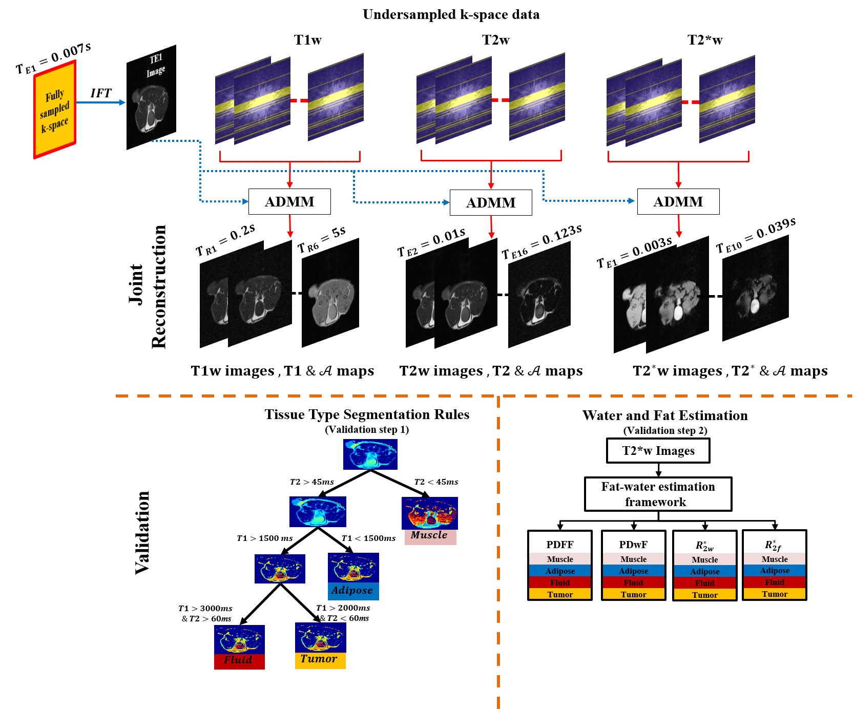
A joint reconstruction framework is proposed to reconstruct a series of T1-weighted, T2-weighted, and T2*-weighted images and corresponding parameter maps simultaneously from undersampled cartesian k-space data. Joint Total Variation (JTV) and model-based constraints were employed to resolve the ambiguity introduced due to undersampling. T1 and T2 maps were used to identify fluid, adipose, muscle and tumor tissue types. T2*w images reconstructed from undersampled data were analyzed to produce maps of Proton Density Fat Fraction (PDFF), Proton Density Water Fraction (PDwF), and the relaxation rates of water ($$$R^*_{2w}$$$) and fat ($$$R^*_{2f}$$$) in each tissue type [1].
Purpose
MRI offers excellent soft-tissue contrast, and the option of varying the contrast observed between tissues, by varying the type of acquisition, e.g., T1, T2 and T2* weighted, even without the use of exogenously administered contrast agents. To make quantitative image information comparable across patients and scan dates it is often preferable to acquire parameter maps (e.g., T1, T2, T2*, and proton density maps). Co-registered multiparametric MRI (mpMRI) images and parameter maps are amenable to multispectral analysis to objectively identify various tissue types to assist differential diagnosis, identify tumors and their evolution in response to therapies, and to predict patient outcomes [2-6]. However, the sequential acquisition of mpMRI images and parameter maps is potentially time-consuming, and techniques to accelerate this process are desirable. Least-squares based approaches along with regularizers such as Total Variation (TV), low rank approximation, model-based priors, and sparsity-based priors have been employed to accelerate the reconstruction of multicontrast images and generate the corresponding parametric maps from undersampled k-space data [7-10]. Our hypotheses are, that co-registered T1, T2 and T2* weighted images share significant amounts of structural information, and, each series must follow either a longitudinal or transverse relaxation model. Using these two hypotheses as regularizers, in addition to a least-squares data consistency term, we have simultaneously estimated a series of T1, T2 and T2* weighted images, and the corresponding parameter maps of T1, T2 and T2*, from undersampled k-space date. Reconstructed images and parameter maps were used to compute tissue type maps and maps of PDFF and PDwF, $$$R^*_{2w}$$$ and $$$R^*_{2f}$$$ compared against ground truth.Method
K-space data for six tumor-bearing mice corresponding to T1-weighted (variable TR), T2-weighted (multi-echo spin-echo), and T2*-weighted (multi-echo gradient-echo) sequences were acquired at 7T. It is proposed to reconstruct T1w images $$$u$$$ of size $$$N1 \times N2 \times M$$$ , the corresponding proton density map $$$ A^{T1}$$$ and T1 map of size $$$N1 \times N2$$$ simultaneously. Corresponding to this, an objective function comprising of a data consistency least-squares term, joint total variation term, and magnetization relaxation model based on the longitudinal/transverse relaxation spin, is formulated as in equation 1.$$\underset{u^m \in\mathbb{C}^{N1 \times N2},\mathcal{A^{T1}},T_1 \in \mathbb{R}^{N1 \times N2}}{min}\sum_{m=1}^{M}\frac{||SFu^{(m)}- k^{(m)}||_2^2}{2} + \alpha_1 ||[\mathcal{D}u]^{(m)}||^1_1 \\ + \alpha_2 |||u^{(m)}| -\mathcal{A^{T1}}(1-exp(-t_m/T_1)||_2^2 \hspace{1cm} where [\mathcal{D}u]^{(m)} = \frac{\eta |\nabla u^{(m)}|}{\sqrt{|\nabla v^{(m)}|^2+\eta^2}} ....(1)$$
The first term is the data consistency term. Here $$$S$$$ is the sampling mask and $$$F$$$ represents the 2D FFT function. The next constraint is the Joint Total Variation (JTV) term. Here, $$$v$$$ is the 1st echo of the T2w images which is used to improve the confidence of the edge location in the JTV algorithm[11] and $$$\eta$$$ is a weighting parameter . Finally, a model-based prior based on the longitudinal relaxation of spins is used. Here $$$t_m$$$ is the repetition time and $$$ \alpha_{1} , \alpha_{2}$$$ Lagrangian coefficients. This formulation is solved iteratively using the ADMM algorithm[12]. The proposed algorithm is repeated to reconstruct a series of T2w/T2*w images and the corresponding T2/T2* map with prior based on the transverse relaxation of spin. Finally, validation of T1w and T2w reconstructions is carried out using tissue type segmentation as shown in Figure 1 to objectively identify fluid, adipose, muscle and tumor. Validation of T2*w images was carried out by fitting them according to [1] and calculating the mean PDFF, PDwF, $$$R^*_{2w}$$$ and $$$R^*_{2f}$$$ in each tissue type. Results from undersampled reconstructions are compared against ground truth results from fully-sampled data.
Results and Discussion
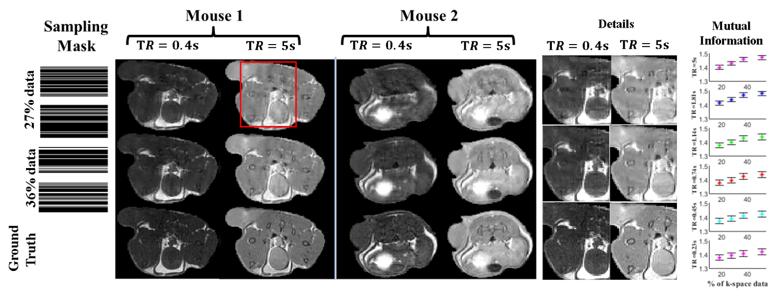
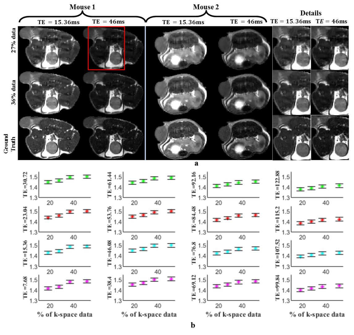
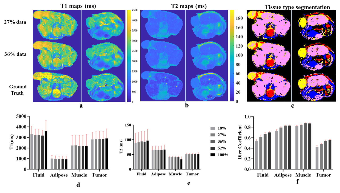
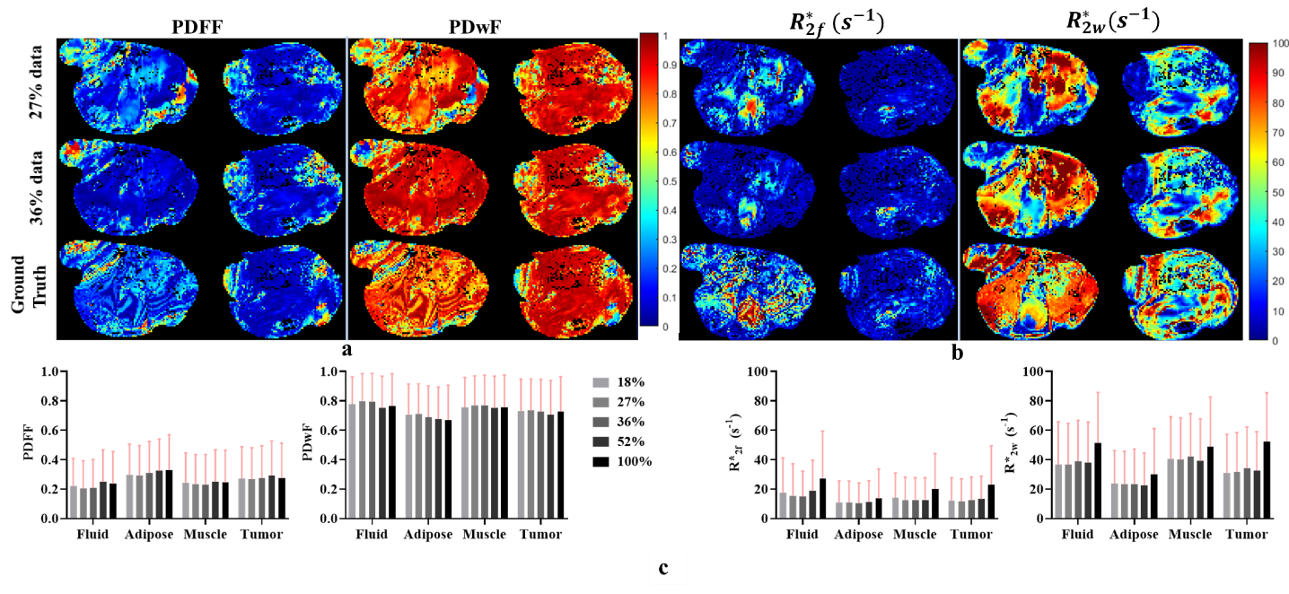
Figures 2 & 3 show the reconstructed images and Mutual Information(MI) for T1w &T2w images respectively. MI values are found to increase as k-space data increases, up to a point. Higher MI values are obtained for longer TR and shorter TE times, which may be due to higher signal-to-noise ratio (SNR) in these images. Figures 4a and 4b show example reconstructed T1 and T2 maps, respectively. Despite some loss of fidelity vis-à-vis the ground truth T1 and T2 maps, tissue type maps computed from undersampled T1 and T2 maps show excellent agreement with tissue type maps computed from fully-sampled T1 and T2 maps (Figure 4c).The mean and standard deviation (SD) of T1 & T2 values in each tissue type and the Dice coefficient are shown in Figure 4d, 4e and 4f respectively. Here, SD represents the true heterogeneity of T1 and T2 values within a given tissue type. Expectedly, Dice coefficients are found to increase as amount of k-space data used increases. Figure 5a and 5b shows the estimated PDFF, PDwF, $$$R^*_{2w}$$$ and $$$R^*_{2f}$$$ for two different mouse slices. Some loss of fidelity may be observed in their estimates, however key features are preserved. The mean and SD values of the estimated parameters in different tissue types are shown in Figure 5c. While, PDFF and PDwF values are found as expected, the relationship between $$$R^*_{2w}$$$ and $$$R^*_{2f}$$$ is unexpected, which may be due to susceptibility effects dominating both relaxation rates.Conclusion
A series of T1w, T2w and T2*w images and the corresponding parameter maps were concurrently reconstructed using the proposed framework. Tissue type maps, PDFF and PDwF within each tissue type computed from 18% k-space data showed good similarity with the fully-sampled ground truth values.Acknowledgements
References
[1] V. V. Chebrolu et al., "Independent estimation of T2* for water and fat for improved accuracy of fat quantification," Magn Reson Med, vol. 63, no. 4, pp. 849-57, Apr 2010.
[2] J. Gohagan et al., "Multispectral analysis of MR images of the breast," vol. 163, no. 3, pp. 703-707, 1987.
[3] M. W. Vannier, R. L. Butterfield, D. L. Rickman, D. M. Jordan, W. A. Murphy, and P. R. J. C. r. i. b. e. Biondetti, "Multispectral magnetic resonance image analysis," vol. 15, no. 2, p. 117, 1987.
[4] T. Taxt, A. Lundervold, B. Fuglaas, H. Lien, and V. J. M. R. i. M. Abeler, "Multispectral analysis of uterine corpus tumors in magnetic resonance imaging," vol. 23, no. 1, pp. 55-76, 1992.
[5] R. A. Carano et al., "Quantification of tumor tissue populations by multispectral analysis," vol. 51, no. 3, pp. 542-551, 2004.
[6] O. Stringfield et al., "Multiparameter MRI Predictors of Long-Term Survival in Glioblastoma Multiforme," vol. 5, no. 1, p. 135, 2019.
[7] L. I. Rudin, S. Osher, and E. Fatemi, "Nonlinear total variation based noise removal algorithms," Physica D: nonlinear phenomena, vol. 60, no. 1-4, pp. 259-268, 1992.
[8] J. Huang, C. Chen, and L. Axel, "Fast multi-contrast MRI reconstruction," Magn Reson Imaging, vol. 32, no. 10, pp. 1344-52, Dec 2014.
[9] J. Yao, Z. Xu, X. Huang, and J. Huang, "An efficient algorithm for dynamic MRI using low-rank and total variation regularizations," J Medical image analysis, vol. 44, pp. 14-27, 2018.
[10] K. T. Block, M. Uecker, and J. Frahm, "Model-based iterative reconstruction for radial fast spin-echo MRI," IEEE transactions on medical imaging, vol. 28, no. 11, pp. 1759-1769, 2009.
[11] M. J. Ehrhardt and M. M. Betcke, "Multicontrast MRI reconstruction with structure-guided total variation," J SIAM Journal on Imaging Sciences, vol. 9, no. 3, pp. 1084-1106, 2016.
[12] S. Boyd, N. Parikh, and E. Chu, "Distributed optimization and statistical learning via the alternating direction method of multipliers," Foundations and Trends in Machine Learning, vol. 3, 2010.
Figures