1186

Automatic WaveCS reconstruction

Gabriel Varela-Mattatall^1,2 and Ravi S Menon^1,2
¹Centre for Functional and Metabolic Mapping, Robarts Research Institute, Western University, London, ON, Canada, ²Department of Medical Biophysics, Schulich School of Medicine and Dentistry, Western University, London, ON, Canada

Synopsis

WaveCS is the combination of corkscrew trajectories in k-space with the application of compressed sensing reconstruction. However, its accurate reconstruction depends critically on user-defined tuning. This is a tedious process that may require additional optimization if acquisition parameters are changed. Furthermore, an incorrect regularization weighting could generate noise amplification, emergence of artifacts, smoothing and loss of structural information. Here, we present a fast, non-iterative and automatic procedure that estimates the regularization weighting and which reconstruction is comparable to previous reconstructions using more tedious approaches that are considered the state-of-the-art.

Purpose

Most compressed sensing¹ (CS) MRI reconstructions^2–10,
$$ \hat{x} = \textrm{argmin} _x \ \ \| Ax - y \|_2^2 + \lambda \| \Psi x \|_1, \hspace{2cm} \textrm{(1)}$$ are based on a data consistency term and a regularization term. The data consistency (first term of Eq. (1)) makes the reconstruction, $$$ x $$$, to resemble the acquired k-space data, $$$ y $$$, after the net sampling operator, $$$ A $$$. The regularizer (second term) promotes sparsity from the reconstruction using an sparsifying transform, $$$ \Psi $$$. One of the problems using Eq. (1), is the determination of the regularization weighting, $$$ \lambda $$$. An incorrect $$$ \lambda $$$ can easily generate artifacts, smoothing, and loss in both structural information as in noise suppression. To assure its correct selection, most CS MRI reconstructions rely on the evaluation of multiple reconstructions to determine $$$ \lambda $$$. In the case of Wave-CAIPI¹¹ using CS-based reconstruction, which is known as WaveCS⁷,
$$ \hat{x} = \textrm{argmin} _x \ \ \| SF_jkPF_iCx - y \|_2^2 + \lambda_g \| G x \|_1 + \lambda_w \| W x \|_1, \hspace{2cm} \textrm{(2)}$$
the original optimization problem considers two regularizers. For the sake of simplicity, previous work assumed $$$ \lambda_g = \lambda_w $$$ and did multiple evaluations using the normalized mean squared error and the fully sampled k-space to obtain their results, but this methodology is not realistic for prospective under-sampled acquisitions. Furthermore, any change in the acquisition and reconstruction will often require retuning $$$ \lambda $$$. Here, we show that we can re-write Eq. (2) as,
$$ \hat{x} = \textrm{argmin} _x \ \ \| SF_jkPF_iCx - y \|_2^2 + \lambda_{\textrm{auto}} \| W x \|_1, \hspace{2cm} \textrm{(3)}$$
and we show that Eq. (3) provides an automatic approach to obtain the regularization weighting, which enables an automatic WaveCS reconstruction.

Theory

Our approach to determine the automatic regularization weighting, $$$ \lambda_{\textrm{auto}} $$$ from Eq. (3), can be described in two main steps.
1- Estimation of the maximum decomposition level for the wavelet transform:
We measure sparsity per decomposition level by means of the Gini index¹² and determine the maximum decomposition level by increasing the decomposition level until the Gini index for the next level decreases.
2- Determination of level-dependent regularization weighting:
We define a level-dependent regularization weighting as the boundary between the body and the tails of each wavelet coefficients’ histogram using a $$$k$$$-means algorithm ($$$k$$$=2). The feature for allocation is the frequency from each histogram. Without loss of generality, the typically scalar value of $$$ \lambda_{\textrm{auto}} $$$ in Eq. (3), can also be a diagonal matrix. Thus, the soft-thresholding function, which is the proximal operator^13,14 of the regularizer in Eq. (3), $$$ \lambda_{\textrm{auto}} \| W x \|_1 $$$, can be performed level-wise.

Methods

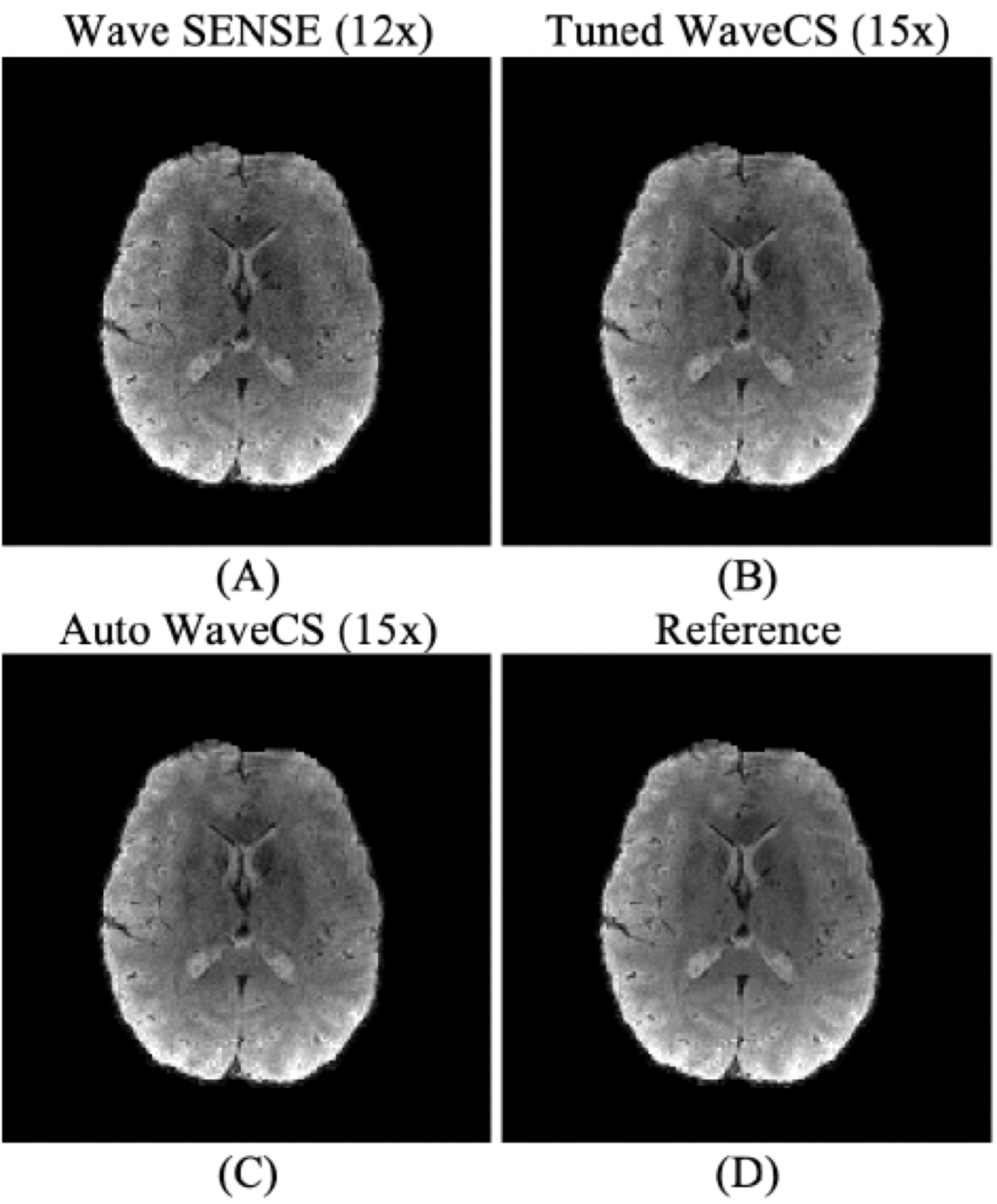
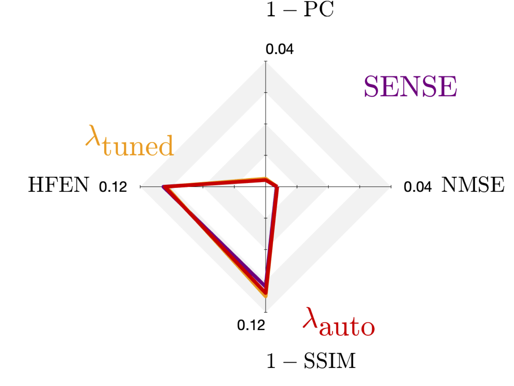
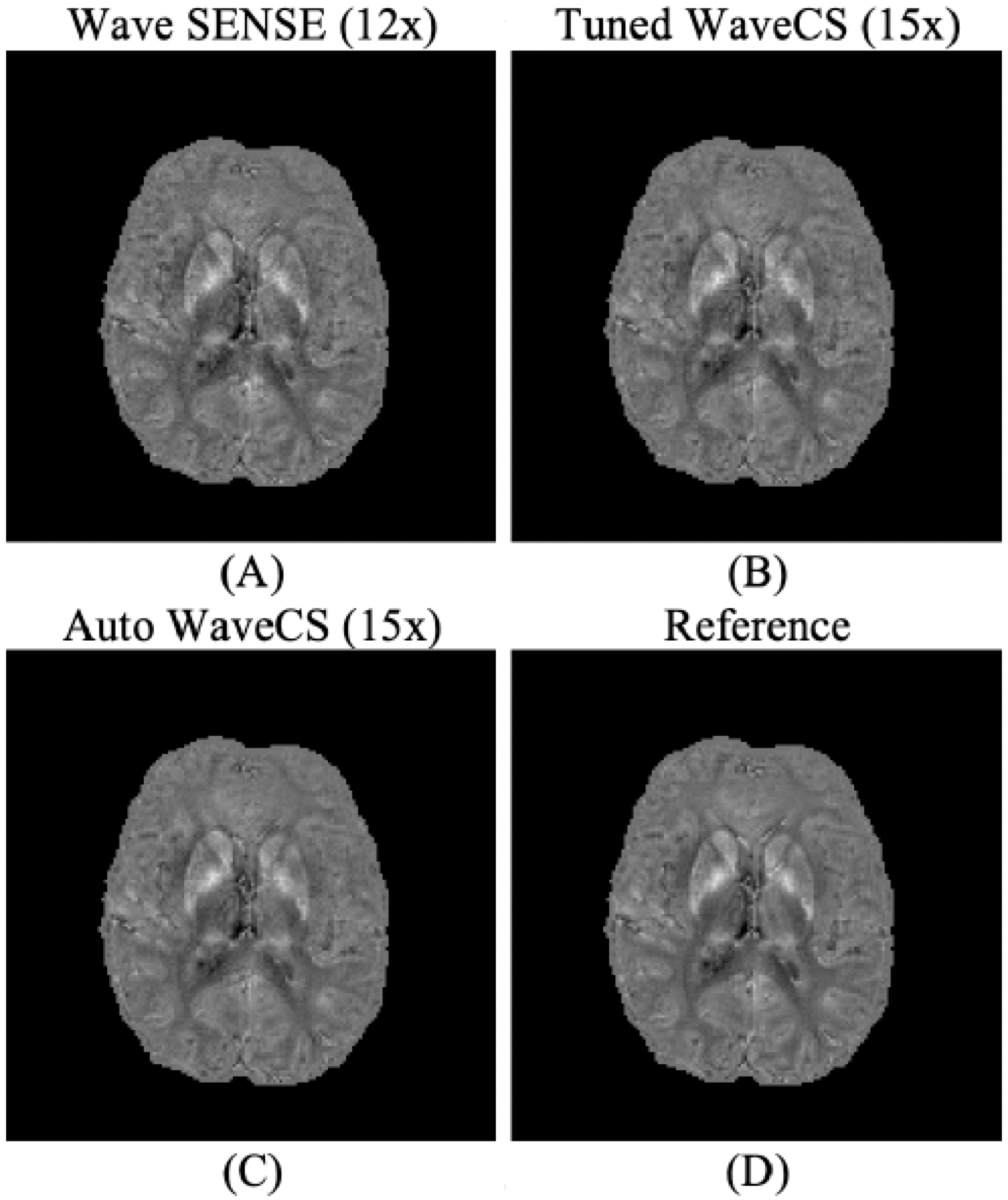
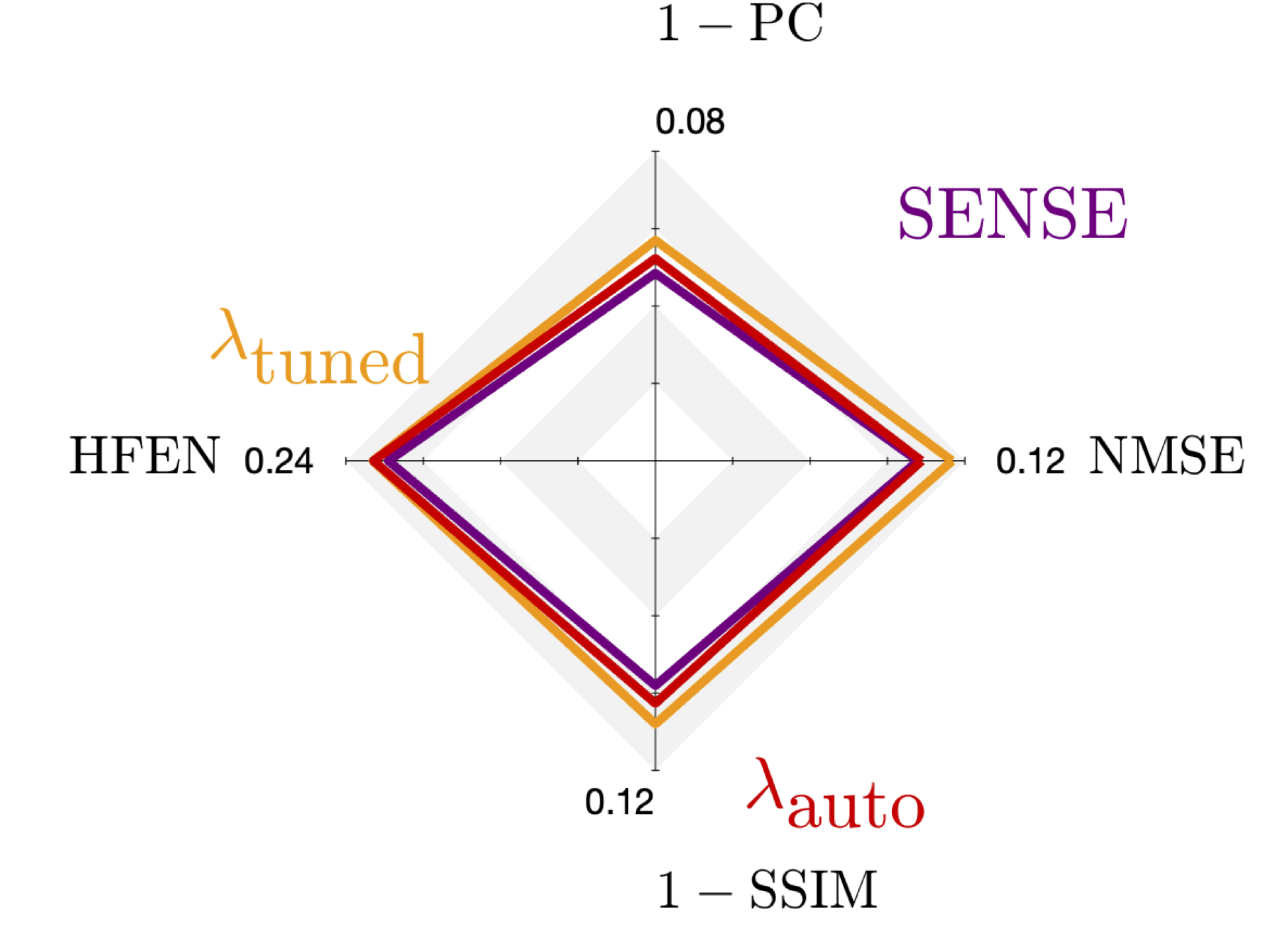
Using the dataset and Matlab codes from (https://www.dropbox.com/s/py1vt8akufkcmzf/CS_Wave_Toolbox.zip?dl=0), we compare the results obtained in Bilgic et al⁷ using Wave Sense and tuned WaveCS, $$$ \lambda_{\textrm{tuned}} $$$, to our automatic WaveCS, $$$ \lambda_{\textrm{auto}} $$$. Wave Sense reconstruction is done with an under-sampling factor of 12x; meanwhile, CS-based reconstructions are done with an under-sampling factor of 15x. For auto WaveCS reconstruction, Eq. (3), we use our own implementation of FISTA and using the 4th Daubechies mother wavelet as the sparsifying transform. The fully sampled image is used as a reference.
Both qualitative and quantitative assessment of complex reconstructions are done through their respective magnitude and phase images. Prior to analyzing phase images, we did Laplacian unwrapping and V-SHARP procedures, as in Bilgic et al⁷, in order to analyze their local phase. To evaluate the comparison between magnitude and local phase images to the ones obtained from the reference, we use the normalized mean squared error (NMSE), Pearson’s correlation coefficient (PC), high-frequency error norm (HFEN)¹⁵ and structural similarity index (SSIM)¹⁶ as reconstruction quality indices.

Results

Figures 1-4 show that there is no practical difference between the different reconstruction methods. It is noteworthy that while Wave SENSE has a slightly better resemblance to the reference, the under-sampling factor for it is of 12x while CS-based strategies use an under-sampling factor of 15x. Between the two Wave CS-based optimization procedures, our proposal is automatic, non-iterative, and the time required to determine the regularization weighting for a 160x160x90 volume is 2.85 seconds.

Conclusion

Our automatic procedure to reconstruct WAVE-CAIPI k-space data is in the same order of error as previous state-of-the-art reconstruction procedures. Future work would focus on implementing the corkscrew trajectory and analyze the effect of prospective under-sampling for this method.

Acknowledgements

Authors wish to acknowledge funding from CIHR Grant FRN 148453 to RSM and BrainsCAN-the Canada First Research Excellence Fund award to Western University

References

1. Candes EJ, Wakin MB. An Introduction To Compressive Sampling. IEEE Signal Process Mag. 2008;25(2):21-30. doi:10.1109/MSP.2007.9147312.

2. Lustig M, Donoho D, Pauly JM. Sparse MRI: The application of compressed sensing for rapid mr imaging. Magn Reson Med. 2006;58:1182–1195.3.
3. Menzel M, Tan Ek, Sperl J, King K et al. Accelerated Diffusion Spectrum Imaging in the Human Brain Using Compressed Sensing. Magn Reson Med. 2011;66:1226–1233.4.
4. Bilgic B, Setsompop K, Cohen-Adad J, Wedeen V, Wald LL, Adalsteinsson E. Accelerated diffusion spectrum imaging with compressed sensing using adaptive dictionaries. Med Image Comput Assist Interv. 2012;15:1–9.5.
5. Paquette M, Merlet S, Gilbert G, Deriche R, Descoteaux M. Comparison of Sampling Strategies and Sparsifying Transforms to Improve Compressed Sensing Diffusion Spectrum Imaging. Magn Reson Med. 2015;73:401–416.6.
6. Otazo R, Candès E, Sodickson DK. Low-rank plus sparse matrix decomposition for accelerated dynamic MRI with separation of background and dynamic components. Magn Reson Med. 2015;73(3):1125-1136. doi:10.1002/mrm.252407.
7. Bilgic B, Ye H, Wald LL, Setsompop K. Simultaneous Time Interleaved MultiSlice (STIMS) for Rapid Susceptibility Weighted acquisition. NeuroImage. 2017;155:577-586. doi:10.1016/j.neuroimage.2017.04.0368.
8. Ong F, Cheng JY, Lustig M. General phase regularized reconstruction using phase cycling. Magn Reson Med. 2018;80(1):112-125. doi:10.1002/mrm.270119.
9. Milovic C, Bilgic B, Zhao B, Acosta‐Cabronero J, Tejos C. Fast nonlinear susceptibility inversion with variational regularization. Magn Reson Med. 2018;80(2):814-821. doi:10.1002/mrm.2707310.
10. Varela‐Mattatall G, Castillo‐Passi C, Koch A, et al. MAPL1: q-space reconstruction using -regularized mean apparent propagator. Magn Reson Med. n/a(n/a). doi:10.1002/mrm.2826811.

11. Bilgic B, Gagoski BA, Cauley SF, et al. Wave-CAIPI for Highly Accelerated 3D Imaging. Magn Reson Med Off J Soc Magn Reson Med Soc Magn Reson Med. 2015;73(6):2152-2162. doi:10.1002/mrm.2534712. 12. Hurley NP, Rickard ST. Comparing Measures of Sparsity. ArXiv08114706 Cs Math. Published online April 27, 2009. Accessed April 12, 2020. http://arxiv.org/abs/0811.470613.

13. Combettes PL, Pesquet J-C. Proximal Splitting Methods in Signal Processing. In: Bauschke HH, Burachik RS, Combettes PL, Elser V, Luke DR, Wolkowicz H, eds. Fixed-Point Algorithms for Inverse Problems in Science and Engineering. Vol 49. Springer Optimization and Its Applications. Springer New York; 2011:185-212. doi:10.1007/978-1-4419-9569-8_1014.

14. Boyd S. Neal Parikh Department of Computer Science Stanford University. :113.15.

15. Langkammer C, Schweser F, Shmueli K, et al. Quantitative Susceptibility Mapping: Report from the 2016 Reconstruction Challenge. Magn Reson Med. 2018;79(3):1661-1673. doi:10.1002/mrm.2683016. 16. Zhou Wang, Bovik AC, Sheikh HR, Simoncelli EP. Image quality assessment: from error visibility to structural similarity. IEEE Trans Image Process. 2004;13(4):600-612. doi:10.1109/TIP.2003.819861

Figures

Visualization of magnitude Images from the different reconstruction procedures. Panels (A) and (B) show the results from Bilgic et al⁷, while panel (C) shows the result from our automatic WaveCS reconstruction. Panel (D) shows the reference. In parenthesis it is shown the under-sampling factor for each reconstruction.

Quantitative analysis from magnitude images of the different reconstruction procedures. We compare the quantitative results from Wave SENSE, a tuned version of WaveCS, $$$ \lambda_{\textrm{tuned}} $$$, and our automatic version of WaveCS, $$$ \lambda_{\textrm{auto}} $$$, to the reference. Smaller values along each axis represent more accurate reconstructions.

Visualization of local phase images from the different reconstruction procedures. Panels (A) and (B) show the local phase from Bilgic et al⁷, while panel (C) shows the local phase obtained from our automatic WaveCS reconstruction procedure. Panel (D) shows the reference. In parenthesis it is shown the under-sampling factor for each reconstruction.

Quantitative analysis from local phase images of the different reconstruction procedures. We compare the quantitative results from Wave SENSE, a tuned version of WaveCS, $$$ \lambda_{\textrm{tuned}} $$$, and our automatic version of WaveCS, $$$ \lambda_{\textrm{auto}} $$$, to the reference. Smaller values along each axis represent more accurate reconstructions.

Proc. Intl. Soc. Mag. Reson. Med. 29 (2021)

1186