Introduction

Compressed sensing (CS) allows a reduction in scan time at the cost of longer reconstruction times. Preconditioning techniques can shorten these reconstruction times by reducing the number of iterations that are needed to converge to the optimal image solution [1,2,3]. However, designing an efficient preconditioner is not straightforward, since it is often hard to approximate the inverse operation of the signal model of interest in a computationally inexpensive manner. Deep learning reconstruction approaches, on the other hand, are often inherently fast [4], with the additional advantage of not needing to tune regularization parameters of the CS formulation. While the latter class has shown great reconstruction performance over the past years, a disadvantage is the risk of the trained network not generalizing well to unseen or abnormal anatomies, and the lack of understanding and detecting corresponding image artifacts. In this work, we aim to integrate deep learning in a classical CS reconstruction approach: we explore the feasibility of learning a preconditioner for CS using a convolutional neural network. The evaluation of such a preconditioner will be fast and can support reconstruction acceleration without introducing uncertainty to the reconstruction quality.

Methods

We train a network that learns the inverse operation $$$M\approx A^{-1}$$$ of the linear system in Split Bregman (SB) [5]
$$\mathbf{y}=\sum_{i=1}^{N_c} (RFS_i)^H \mathbf{y}_i =\{ \sum_{i=1}^{N_c} (RFS_i)^HRFS_i+\lambda (D_x^HD_x + D_y^HD_y)+\gamma W^HW \} \mathbf{x} =A\mathbf{x} $$
such that $$$M\mathbf{y}=MA\mathbf{x}\approx \mathbf{x}$$$, with $$$\mathbf{x}$$$ the unknown image, $$$\mathbf{y}_i$$$ the acquired k-space data for coil $$$i$$$ with coil sensitivity map $$$S_i$$$, $$$R$$$ the sampling mask, $$$F$$$ the uniform Fourier transform, $$$D_x,D_y$$$ finite difference operators and $$$W$$$ a wavelet transform (Daubechies-4). Instead of learning a matrix $$$M$$$, we design the model such that the network learns the action of a preconditioner $$$M$$$ on a vector $$$\mathbf{y}$$$, which makes using the learned preconditioner computationally inexpensive (~0.03s per evaluation).

Simulation of training examples: To avoid explicitly calculating the inverse of a large dense matrix for each training example, the network’s input images $$$\mathbf{y}^{[k]}$$$ were computed from the labels $$$\mathbf{x}^{[k]}$$$ using the forward operator $$$A$$$ such that $$$\mathbf{y}^{[k]} =A\mathbf{x}^{[k]}$$$. The training set was constructed from an equal amount of complex white noise and brain images (Human Connectome Project) with matrix size 128x128. The $$$\mathbf{x}^{[k]}$$$ set was augmented by rotating each image four times in steps of 90 degrees, after which a Gaussian-shaped phase was randomly added to each image. This resulted in 53160 $$$\mathbf{x}^{[k]}$$$. Corresponding $$$\mathbf{y}^{[k]}$$$ were simulated for each $$$\mathbf{x}^{[k]}$$$ with an undersampling factor between 1 and 8 and Gaussian-shaped complex coil sensitivity maps for 1 to 16 coil elements. $$$\lambda$$$ and $$$\gamma$$$ were randomly selected from (0,10) and transformed into uniform regularization maps. The $$$\mathbf{y}^{[k]}$$$ were normalized and the $$$\mathbf{x}^{[k]}$$$ accordingly scaled. Images and coil sensitivity maps were split into real and imaginary components, yielding a 37-channel network input.
Model and training: We used a residual neural network with three residual blocks containing two layers each [6]. A 2D convolution (3x3 kernels,128 features) was performed at every layer with ReLu (hidden layers) and tanh (output layer) activations. We minimized the mean squared error over 20 epochs using Adam with an initial learning rate of 5e-4, a batch size of 32 and dropout with a probability of 0.25. Training was performed in Tensorflow with a 12GB gpu.
Data acquisition and image reconstruction: To test the performance of the learned preconditioner in the CS framework, fully sampled and undersampled scans in three healthy volunteers (brain FLAIR, brain TSE, knee FFE) were acquired on an Ingenia 3T dual transmit MR system (Philips Helathcare), with a 15-channel head coil and a 16-channel knee coil (informed consent obtained). Images were reconstructed with SB for two matrix sizes (128x128 and 256x256) with and without the learned preconditioner, and compared to the circulant preconditioner designed in Ref [2].

Results

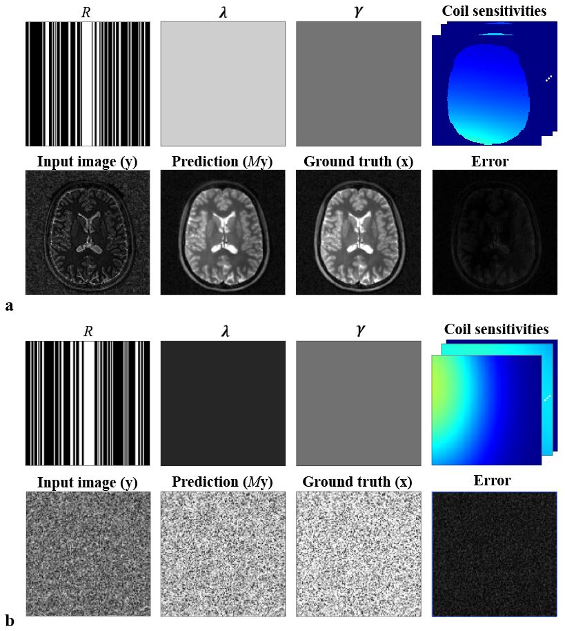
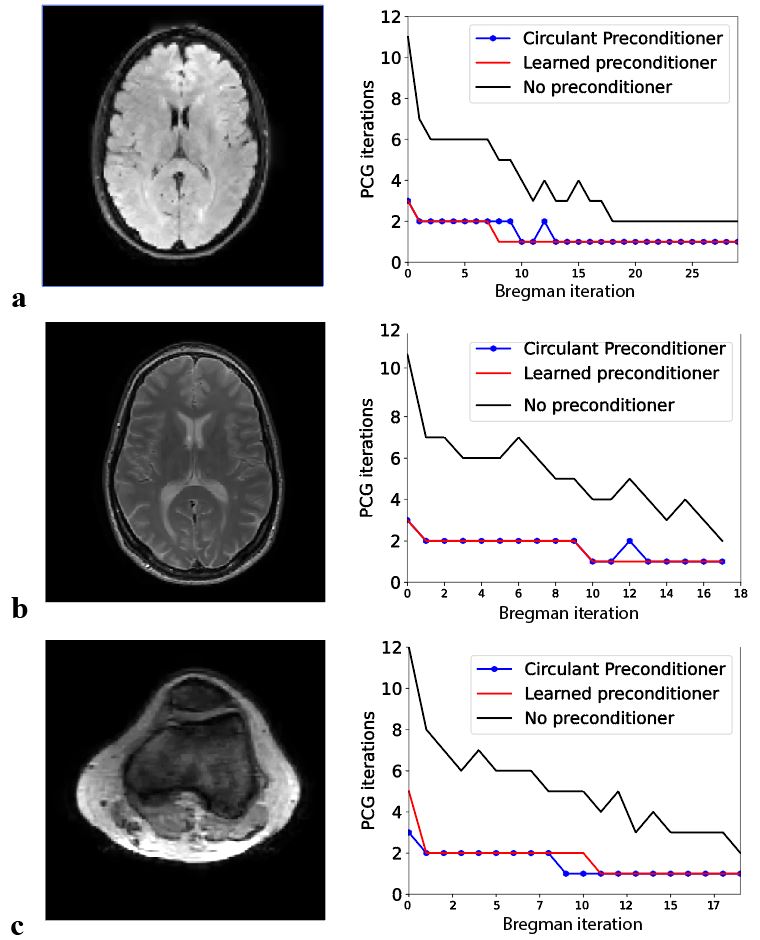
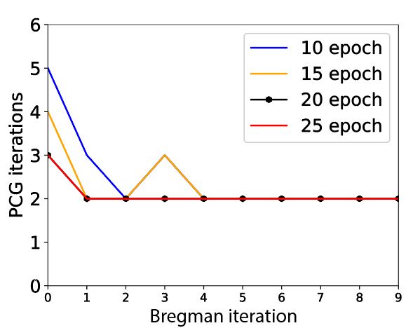
Figure 1 shows the network’s input ($$$R$$$, $$$\lambda$$$, $$$\gamma$$$, coil sensitivities, image) and output for (a) a brain and (b) a noise example. The network’s prediction $$$M\mathbf{y}$$$ of the operation $$$A^{-1}\mathbf{y}$$$ is close to the ground truth image for both cases. This is confirmed by the low absolute errors (normalized norm<0.16). Applying the learned preconditioner to SB results in an acceleration factor of 2.9 in the conjugate gradient (CG) method. Figure 2 shows that it is possible for a learned preconditioner to meet and slightly improve upon the performance of an efficient circulant preconditioner. The performance of the preconditioner is plotted for different number of training epoch in Figure 3, suggesting that there is room for further improvement.

Discussion

The learned preconditioner has shown to accelerate reconstructions for different anatomies, number of coils and undersampling factors ($$$R=2,R=3$$$), which means that it is not necessary to train a new network for each type of scan. The choice of convolutional layers allows the network to generalizes to different resolutions/matrix sizes. The performance is currently slightly better for brain scans than for a knee scan, but optimization of the network architecture and the training set may help to further improve the generalizability.

Conclusion

It is possible to design a preconditioner for CS reconstructions using a convolutional neural network. Such an approach can potentially help to further accelerate CS reconstructions compared to existing preconditioners.

Acknowledgements

This project is funded by NWO-TTW (HTSM-17104). We would like to thank the Division of Image Processing from the Leiden University Medical Center for providing computing recourses.