1169
ZTE Infilling From Auto-calibration Neighbourhood Elements
Tobias C Wood1, Emil Ljungberg1, and Mark Chiew2
1Neuroimaging, King's College London, London, United Kingdom, 2Wellcome Centre for Integrative Neuroimaging, FMRIB, Nuffield Department of Clinical Neurosciences, University of Oxford, Oxford, United Kingdom
1Neuroimaging, King's College London, London, United Kingdom, 2Wellcome Centre for Integrative Neuroimaging, FMRIB, Nuffield Department of Clinical Neurosciences, University of Oxford, Oxford, United Kingdom
Synopsis
We present a method for filling the dead-time gap in ZTE imaging using a parallel imaging technique. We present results in phantoms and a human brain demonstrating high fidelity reconstructions comparable to existing methods that require collection of additional data.
Introduction
The Zero Echo-Time (ZTE) pulse sequence was originally developed to image flowing liquids [1]. Its serendipitous properties include minimal acoustic noise [2] and the ability to capture signals from protons with ultra-short relaxation times [3]. However, as illustrated in figure 1 a TE of 0 cannot be achieved in practice and there is a short dead-time gap of several microseconds. This leads to a few missing samples in the centre of k-space, which can result in large reconstruction artefacts depending on scan parameters. Existing methods to correct this artefact acquire either an extra low-resolution k-space or additional single-point acquisitions [3]. These data points may have different T2* decay or spoiling properties, and hence merging it with the high-resolution k-space data is not always straightforward.Modern MRI scans are generally acquired using multi-channel coils, and parallel imaging exploits data redundancy between these to synthesise deliberately un-acquired k-space data [4]. We hypothesised that parallel-imaging could instead be used to fill the dead-time gap. In this work, we demonstrate the feasibility of this method in phantoms and in-vivo brain images. We name this method ZTE IN-filling From Autocalibration NeighbourhooD ELements (ZINFANDEL).
Methods
To fill the dead-time gap, we reduce the gold-standard GRAPPA framework from two dimensions to one dimension and apply it to each acquired radial spoke, as illustrated in figure 2. Each spoke contains Nr samples across Nc channels, the first Ng points fall in the dead-time gap, and we set Ns to the number of source points for the kernel. We choose the Nl closest points to the dead-time gap to act as the calibration region. In comparison to 2D GRAPPA, Nl is generally quite small so to increase the number of calibration points we use the Nk closest spokes, assuming the kernel only varies slowly in the angular direction.In the calibration step we divide the calibration region into sets consisting of a target point and the contiguous Ns source points and formulate the calibration source S (Nc*Ns by Nl*Nk) and target T (Nc by Nl*Nk) matrices. We then solve for the weight matrix W using the equation
$$
\textbf{T}=\textbf{W}\textbf{S}\quad\quad\quad\quad (1)
$$
In the synthesis step we fill a single point in the gap by applying equation 1 to the Ns closest points. We iterate this process across all spokes and then iterate again until the dead-time gap is completely filled. We empirically found that this looping order, which progressively updates the kernel weights as points are filled, had better performance than training a single kernel per spoke [5].
To demonstrate this method we used a ZTE sequence implemented on a 3T MR750 scanner (GE Healthcare, Chicago, IL) and 32-channel head coil (Nova Medical). We scanned a spherical water phantom at 2 mm isotropic resolution, 220x220x220 mm FoV, FA 1°, with read-out bandwidths of ±41.67 kHz and ±15.625 kHz (2x oversampled) corresponding to dead-time gaps of 3 and 2 samples respectively. We also scanned a volunteer at 3 mm isotropic resolution, 216x216x126 mm FoV, FA 1°, ±31.25 kHz (dead-time gap 3) and separately with a 12-channel head coil and IR-prepared ZTE sequence, 1 mm isotropic resolution, 220 mm isotropic FoV, FA 2°, TI450 ms. All scans were acquired with a low-resolution k-space for comparison [6]. Scans were acquired with an angular under-sampling factor of 𝜋 relative to Cartesian sampling, except the 3 mm scan which had a further factor of 2.
Images were reconstructed using RIESLING (https://github.com/spinicist/riesling). The raw k-space data was first compressed to 16 or 8 channels [7], ZINFANDEL applied using Nk=5, Ns=5, Nl=16, and finally images reconstructed on a 2x oversampled grid and root-sum-squares channel combination [8]. Images were additionally reconstructed both without applying ZINFANDEL and with the low-resolution k-space instead for comparison.
Results & Discussion
Figure 3 shows the water phantom reconstructed at two bandwidths and dead-time gaps. At both bandwidths when the dead-time gap is unfilled a significant artefact manifests as a low-intensity region in the center of the phantom and high intensity outside of the phantom. Filling the dead-time gap with either ZINFANDEL or the low-resolution k-space removes the artefact.Figures 4 & 5 show the brain scan, which show artifactual high intensity in the void spaces when the dead-time gap is unfilled. These are very strong in the 3 mm image, which is also blurred due to the extreme angular under-sampling. ZINFANDEL corrects these artefacts and restores signal to the parenchyma.
There are some residual low spatial frequency differences between ZINFANDEL and the reference low-resolution k-space method. However, these are at least partially to be expected as the low-resolution k-space is acquired with a reduced gradient amplitude. This corresponds to different T2* decay weighting [3], a different slab profile [9], and different spoiling due to the reduced gradient. For the brain scan, no obvious anatomical detail is present in the difference image, suggesting a high fidelity reconstruction with ZINFANDEL.
Conclusion
We have demonstrated that ZINFANDEL is a viable method of filling dead-time gaps up to three samples. Where ZTE scans are acquired with a multi-channel coil this could make ZTE sequences and reconstruction more flexible and straightforward, as no additional data must be acquired.Acknowledgements
This work was supported by the Wellcome/EPSRC Centre for Medical Engineering [WT 203148/Z/16/Z] and the NIHR Clinical Research Facility at King's College Hospital. MC is supported by the Royal Academy of Engineering (RF201617\16\23).References
- Madio, D. P. & Lowe, I. J. Ultra-fast imaging using low flip angles and fids. Magnetic Resonance in Medicine 34, 525–529 (1995).
- Alibek, S. et al. Acoustic noise reduction in MRI using Silent Scan: an initial experience. Diagnostic and Interventional Radiology 20, 360–363 (2014).
- Weiger, M. et al. Advances in MRI of the myelin bilayer. NeuroImage 217, 116888 (2020).
- Griswold, M. A. et al. Generalized autocalibrating partially parallel acquisitions (GRAPPA). Magnetic Resonance in Medicine 47, 1202–1210 (2002).
- Blaimer, M. et al. 2D-GRAPPA-operator for faster 3D parallel MRI. Magnetic Resonance in Medicine 56, 1359–1364 (2006).
- Wu, Y. et al. Water- and fat-suppressed proton projection MRI (WASPI) of rat femur bone. Magnetic Resonance in Medicine 57, 554–567 (2007).
- Huang, F., Vijayakumar, S., Li, Y., Hertel, S. & Duensing, G. R. A software channel compression technique for faster reconstruction with many channels. Magnetic Resonance Imaging 26, 133–141 (2008).
- Oesterle, C., Markl, M., Strecker, R., Kraemer, F. M. & Hennig, J. Spiral reconstruction by regridding to a large rectilinear matrix: A practical solution for routine systems. Journal of Magnetic Resonance Imaging 10, 84–92 (1999).
- Grodzki, D. M., Jakob, P. M. & Heismann, B. Correcting slice selectivity in hard pulse sequences. Journal of Magnetic Resonance 214, 61–67 (2012).
Figures
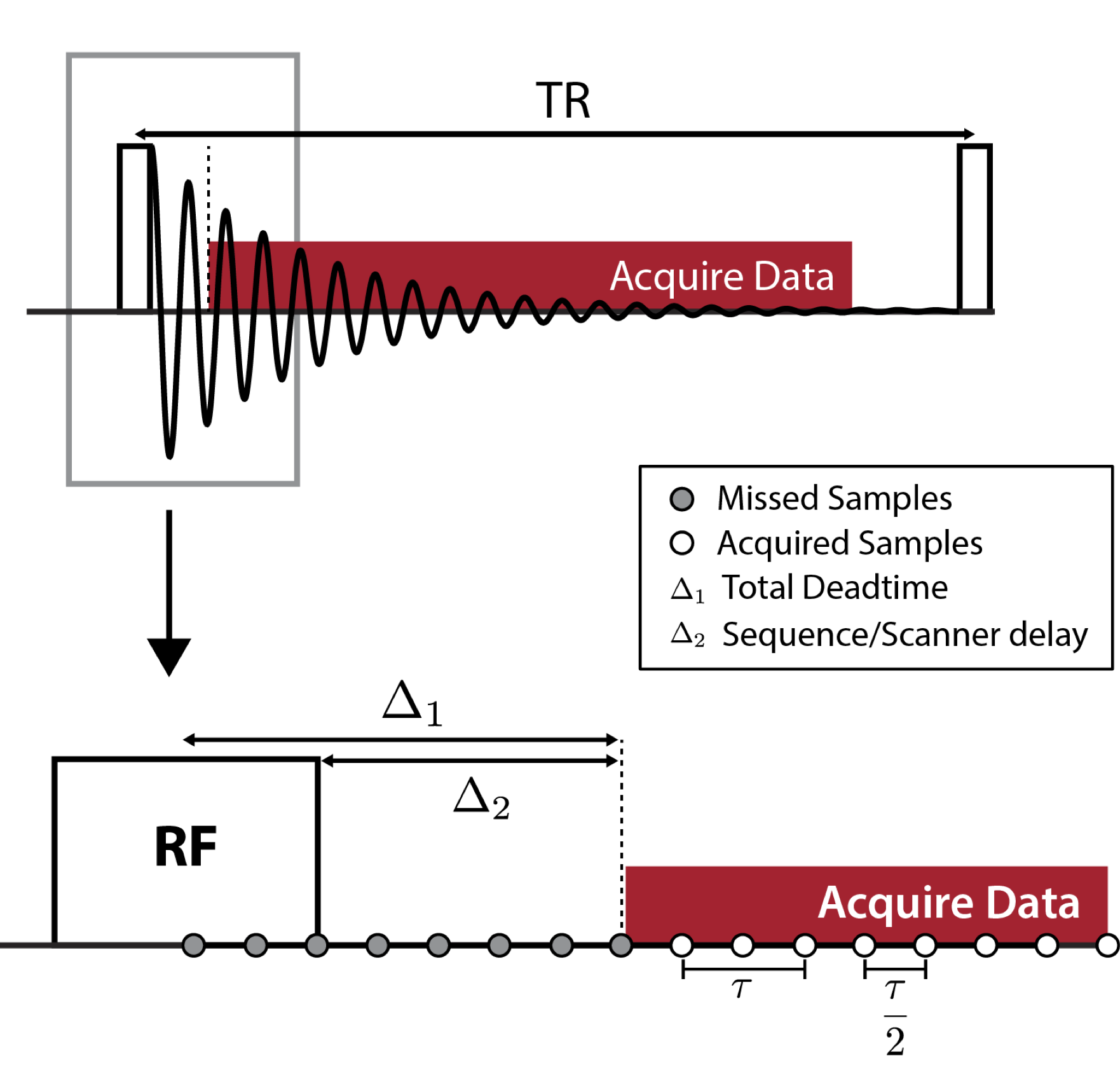
Figure 1: Schematics showing (top) one TR of a ZTE sequence and (bottom) a zoomed-in section showing the dead-time gap between RF excitation and the start of reliable data acquisition. Radial sampling is here exemplified with x2 oversampling, with τ being the dwell time. Reproduced from E. Ljungberg, “MRI with Zero Echo Time: Quick, Quiet, Quantitative,” King’s College London, 2020.
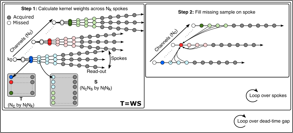
Figure 2: Diagram of the ZINFANDEL algorithm. In step 1, a kernel matrix W is calculated from the calibration region. In step 2, a point in the dead-time gap is filled. By looping first over spokes and then missed samples, the matrix W can be progressively updated towards the center of k-space.
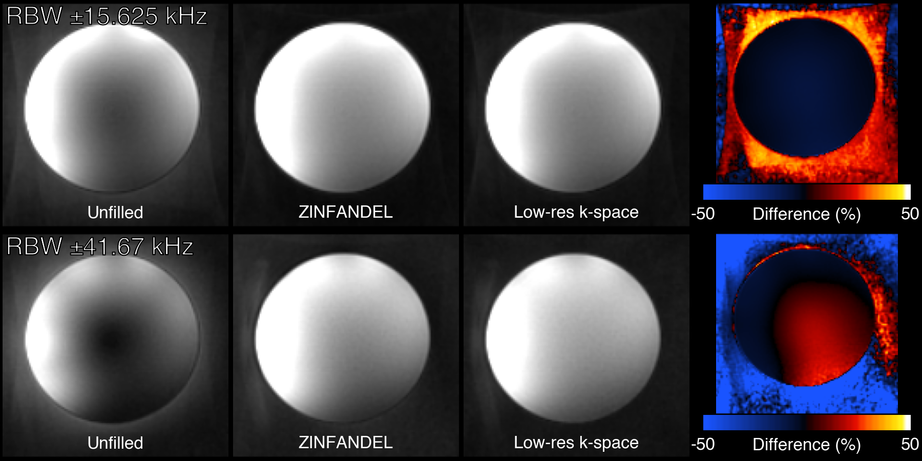
Figure 3: A spherical water phantom scanned at two bandwidths (top row rBW=±15.625 kHz, bottom row rBW=±41.67kHz) and reconstructed without dead-time filling, with ZINFANDEL and with the reference low-resolution k-space method. ZINFANDEL performs equally to the reference.
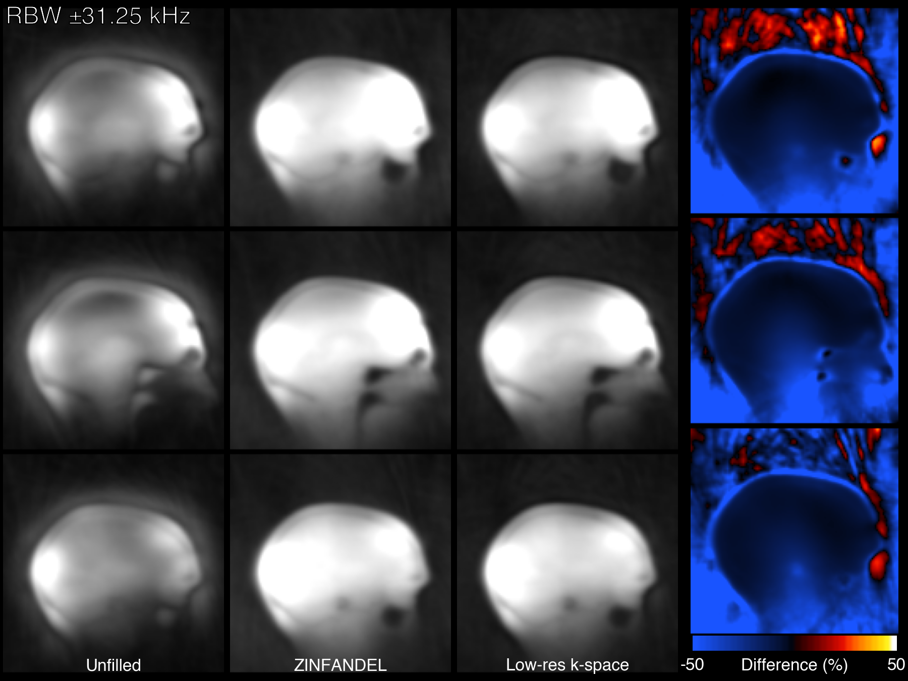
Figure 4: A low-resolution head scan acquired with a fast bandwidth and angular under-sampling. Despite the increased dead-time gap and paucity of calibration data, ZINFANDEL provides an artefact free reconstruction.
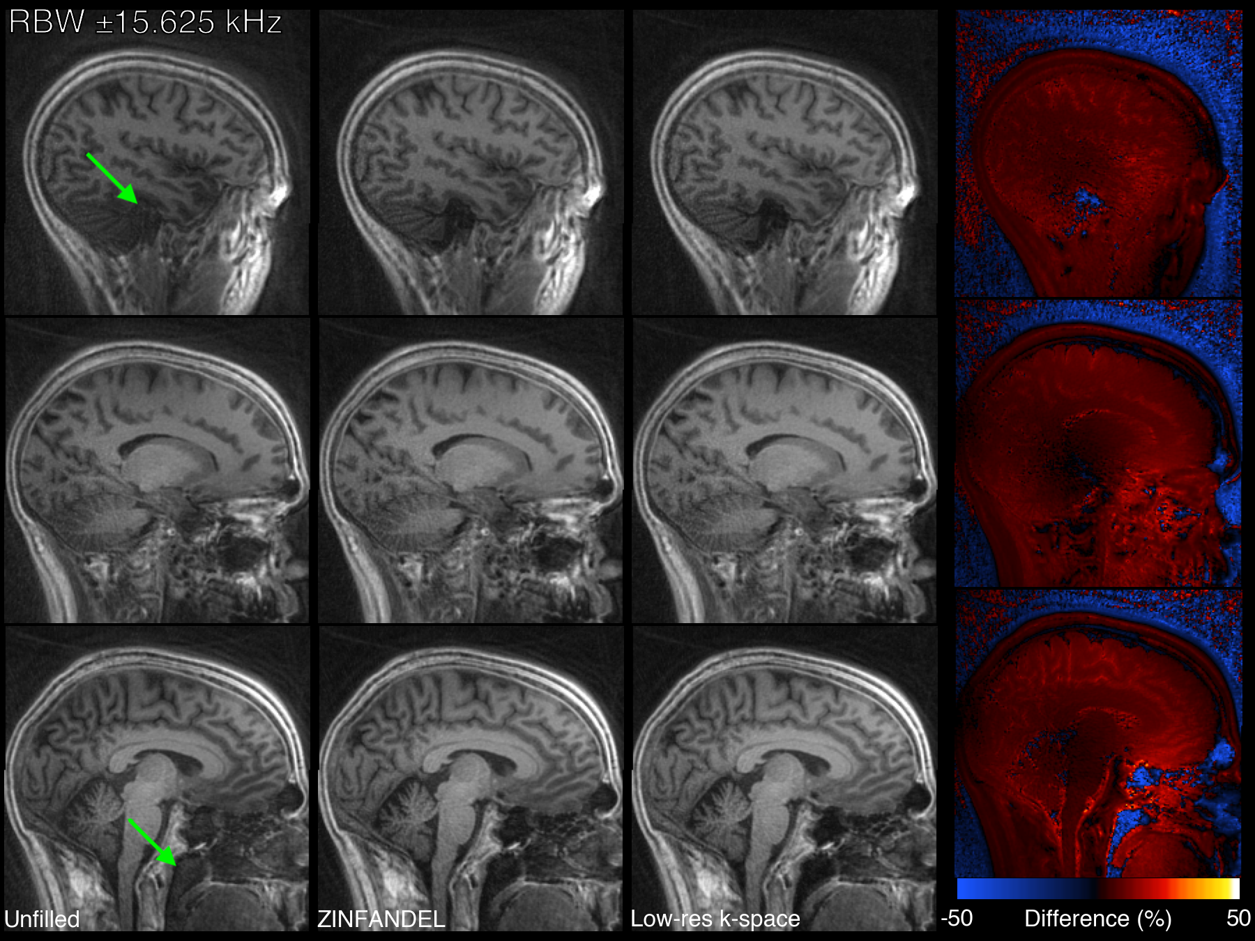
Figure 5: A high-resolution head scan acquired with a 12-channel head coil. ZINFANDEL and the reference method correct the artefacts in the signal voids (green arrows) and show close agreement.