1163
Autocalibrating Segmented Diffusion Weighted Acquisitions (ASeDiWA)
Michael Herbst1
1Bruker BioSpin MRI GmbH, Ettlingen, Germany
1Bruker BioSpin MRI GmbH, Ettlingen, Germany
Synopsis
Segmented EPI enables high resolution DWI. However, phase differences between segments can lead to severe artifacts. This work investigates an algorithm to enable reconstruction of interleaved segmented acquisitions without the need of additional calibration or navigator measurements. Given a limited number of interleaves, the initial phase estimates can be calculated by a traditional parallel imaging reconstruction, using the unweighted scan of the DWI measurement as a reference. The ASeDiWA jointly reconstructs all segments of one DWI frame maintaining their phase information. Therefore, the algorithm allows for an iterative improvement of the phase estimates included in the joint reconstruction.
Introduction
For high resolution diffusion weighted (DW) EPI, interleaved segmentation provides substantially improved image quality. One drawback of such segmentation is the vulnerability to phase fluctuations. Multiplexed sensitivity encoding1 enables robust high-resolution DWI by formulating a joint SENSE reconstruction. Such joint reconstruction was already applied to k-space based algorithms2,3. However, these required navigators to estimate the segments’ phases. In this work, an operator for joint reconstruction of interleaved segmented DW data in k-space without phase navigation is investigated.Methods
Figure 1 visualizes the general idea of the ASeDiWA operator. First, (fig.1a) an ordinary interleaved combination is displayed, leading to substantial ghosting artifacts.Figure 1b shows the GRAPPA reconstruction of each individual segment. Missing samples are reconstructed according to:
$$x_{is0}(r)=\sum_j g_{rji}^*(\widetilde{R}_{rs}x_{js}),\color{white}{.....}[1]$$
where for each segment ($$$s$$$) the nonacquired k-space value at a position $$$r$$$ in the $$$i$$$-th coil $$$x_{is0}(r)$$$ is calculated from the acquired data of all coils of this segment selected by an operator $$$\widetilde{R}_{rs}$$$ about the position $$$r$$$. $$$g_{rji}^*$$$ denotes a set of weights calculated from reference data obtained from the unweighted (B0) scans.
In fig.1c, the ASeDiWA operator reconstructs missing samples in one segment, using data from all segments. For this operation, new reference data are generated by combining the phase information of each segment reconstructed in Eq.1 with the absolute value of the original reference data in image space:
$$x'_{isn}=IFFT\left\{abs\left\{FFT\left\{x_i\right\}\right\}*phase\left\{FFT\left\{x_{isn} \right\}\right\}\right\},\color{white}{.....}[2]$$
where $$$x'_{isn}$$$ is the modified reference data of a segment $$$s$$$ in the $$$i$$$-th coil.
Given the augmented reference data ($$$x'_{isn}$$$) a second calibration is formulated:
$$\min_{g_{risn}}\sum_{p \epsilon Calib}\left\| \sum_t \sum_j g^*_{rjitsn}(\widetilde{R}_{pt}x'_{jtn}) - x'_{isn}(p) \right\|^2,\color{white}{.....}[3]$$
where the operator $$$\widetilde{R}_{pt}$$$ selects sampled k-space locations from all segments and coils about the positions $$$p$$$.
This set of weights ($$$g^*_{rjitsn}$$$) is used for the second reconstruction step:
$$x_{is(n+1)}(r)=\sum_t\sum_j g_{rjitsn}^*(\widetilde{R}_{rt}x_{jt})\color{white}{.....}[4]$$
To reconstruct a k-space location in one segment $$$x_{is(n+1)}(r)$$$, data from all segments are used.
ASeDiWA reconstructs a full k-space dataset for each segment and coil ($$$x_{is(n+1)}(r)$$$), including information of the object phase. Thus, the steps described in Eq. 2-4 can be iterated as denoted by the index n. Note, that the dataset $$$x_{is(n+1)}(r)$$$ is still reconstructed from the acquired data.
Measurements and Simulations
DWI data with 4 interleaves were acquired on a 3T system with 32-channel head coil (Tim Trio, Siemens Healthcare). Settings: TE/TR = 107/4000ms, FOV = 220×220×3.0mm3, Matrix = 256×260, 1 B0 scan, 3 b-values (500, 1000, and 2000 s/mm2). Data were reconstructed using the three algorithms visualized in fig.1.To evaluate the parallel imaging algorithms, g-factor maps were generated. For different segmentation factors (2, 3, and 4), data were reconstructed with GRAPPA, ASeDiWA, and ASeDiWAn (n denoting the number of additional iterations). Simulations were performed on fully sampled FLASH data, acquired on a 7T system with a 4-channel coil (BioSpec, Bruker BioSpin). Settings: TE/TR = 2.576/500ms, FOV = 20×20×1.0mm3, Matrix = 128×128.
DTI processing was applied on a preclinical dataset with different reconstruction settings. Data were acquired on a 9.4T system with a four-channel cryogenic coil (BioSpec , Bruker BioSpin). Settings: TE/TR = 22/2000ms, FOV = 25×25×0.8mm3, Matrix = 128×128×5, 4 segments, 5 B0 scans, b-value 650 s/mm2, 30 directions, with phase navigation.
Results
Figure 2 compares the FFT reconstruction of the human data with the results of the GRAPPA reconstruction and ASeDiWA. For all b-values, the FFT reconstruction shows ghosting. Ghosting is corrected by GRAPPA as well as ASeDiWA. The comparison between GRAPPA and ASeDiWA shows improved results of the ASeDiWA reconstruction.Figure 3 shows results of the g-factor simulations. The left side of each image contains the magnitude image, the right side displays the g-factor maps. From left to right each reconstruction establishes the phase estimate for the following reconstruction step, improving reconstruction results over iterations.
Figure 4 shows fractional anisotropy and corresponding color maps of the preclinical measurement. The first column (a) shows the standard FFT including the phase information of the navigator. In Figure 4b the navigator information was discarded, resulting in ghosting. Figure 4c displays the GRAPPA reconstruction. While artifacts from ghosting are reduced, a substantial loss in SNR can be observed. In fig.4d, ASeDiWA shows improved quality of the DTI maps, compared to GRAPPA. Further improvement can be observed in fig.4e, displaying ASeDiWA2 with two additional iterations.
Discussion
An algorithm for joint reconstruction of segmented DWI without navigators was presented. Phase estimates of each segment were calculated using a kernel calculated from an unweighted scan of the same experiment. Particularly an iterative reconstruction was shown to improve the g-factor and result in robust DWI, even with a small number of receivers. While the number of receivers limits the approach to a few segments, this constraint is relaxed by iteratively improving phase estimates. The method was applied to several in-vivo datasets, rodents as well as human.Conclusion
The presented ASeDiWA algorithm allows for robust reconstruction of segmented DWI data without additional navigation or calibration measurements. In comparison to GRAPPA reconstruction approaches, the method reduces parallel imaging artifacts and improves SNR. An iterative variant was shown to further improve image quality and to provide robust results especially in the case of a small number of receiver channels.Acknowledgements
No acknowledgement found.References
- Chen N, Guidon A, Chang H-C, Song AW. A robust multi-shot scan strategy for high-resolution diffusion weighted MRI enabled by multiplexed sensitivity-encoding (MUSE). NeuroImage. 2013;72:41-47. doi:10.1016/j.neuroimage.2013.01.038 2.
- Dong Z, Wang F, Ma X, et al. Interleaved EPI diffusion imaging using SPIRiT-based reconstruction with virtual coil compression: Compression Accelerated SPIRiT for iEPI DWI. Magn Reson Med. 2018;79(3):1525-1531. doi:10.1002/mrm.26768 3.
- Liu W, Zhao X, Ma Y, Tang X, Gao J-H. DWI using navigated interleaved multishot EPI with realigned GRAPPA reconstruction: Multishot DWI Using Realigned GRAPPA Reconstruction. Magn Reson Med. 2016;75(1):280-286. doi:10.1002/mrm.25586
Figures
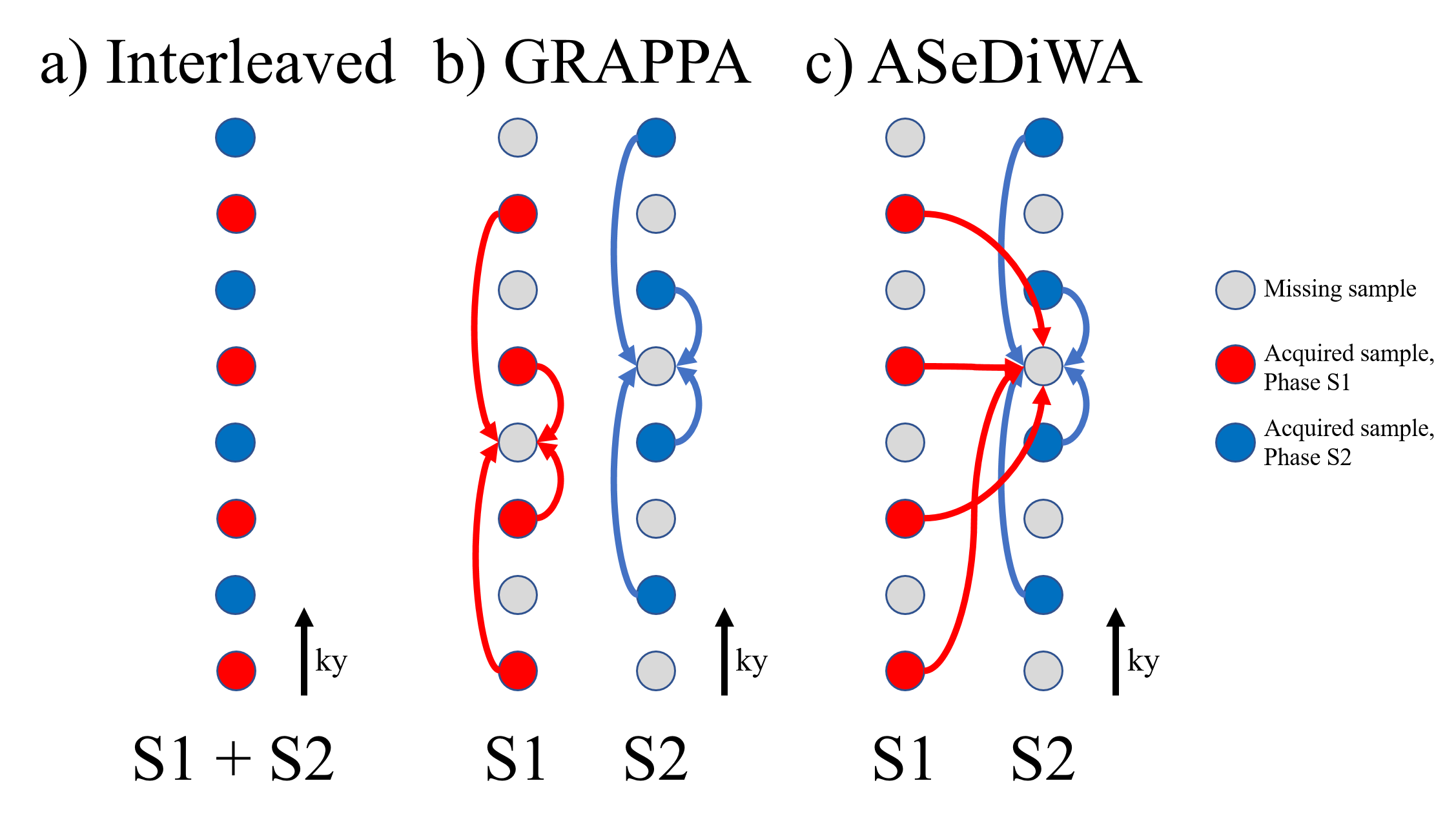
Figure 1: Three options for combining two segments from an interleaved segmented
acquisition are depicted. a: The combination of both segments in one k-space is
shown. Such combination requires phase correction or will lead to strong artifacts in the case of phase differences. b: With GRAPPA, each segment is
reconstructed separately. c: The ASeDiWA algorithm allows the use of acquired
data from all segments to reconstruct the missing samples of each segment.
Note that both reconstructed segments will still have their original phase,
which is required for iterative reconstruction.
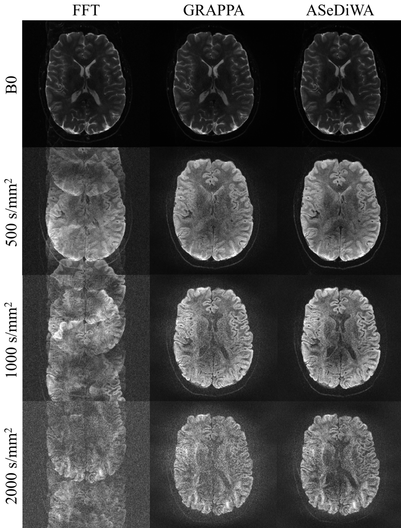
Figure 2: One exemplary slice from the human scan is shown. Each row displays one b-value. In the first column a reconstruction without phase correction is
shown, leading to strong ghosting in the diffusion weighted scans. The second
column shows the GRAPPA reconstruction. The third column displays the ASeDiWA
reconstruction. Both parallel imaging reconstruction methods correct the
ghosting seen in the first column. However, ASeDiWA consistently provides
higher SNR as the GRAPPA reconstruction.
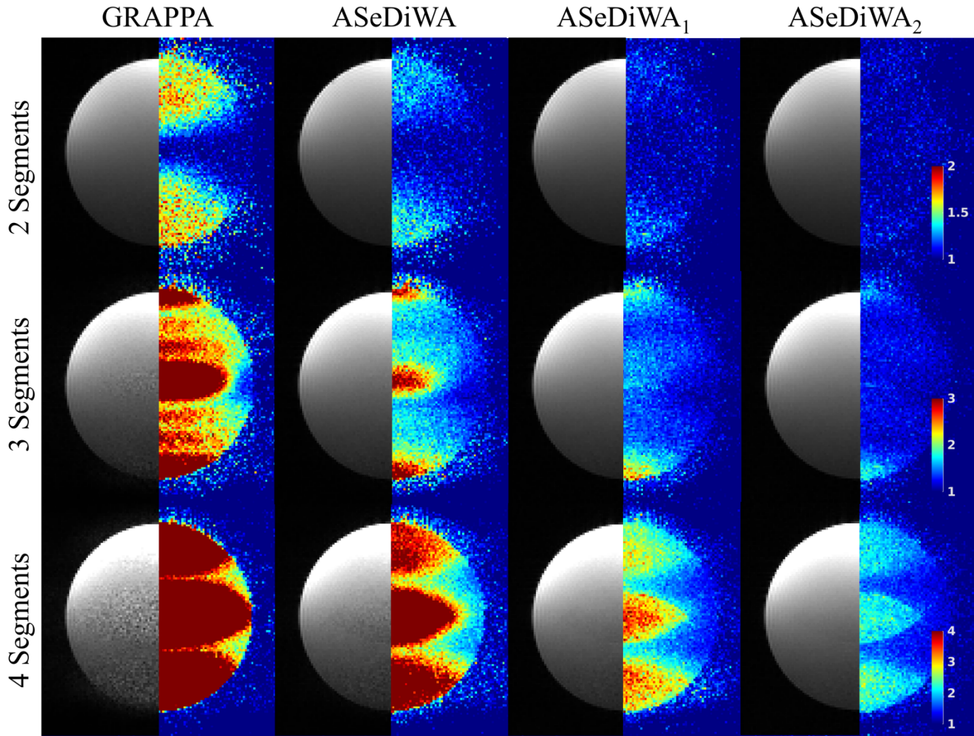
Figure 3: Reconstruction
results (b/w) and g-factor simulations (color) are shown. Each row displays
data with a different number of simulated segments (2, 3, and 4). The first
column shows the data reconstructed with GRAPPA. The following three columns
show results from ASeDiWA without and with one and two iterations,
respectively. In general, higher segmentation leads to higher g-factors.
Independent of the segmentation, the comparison of ASeDiWA with GRAPPA shows a
reduced g-factor. Further improvement can be achieved by iteration of the
algorithm (ASeDiWA1 and ASeDiWA2).
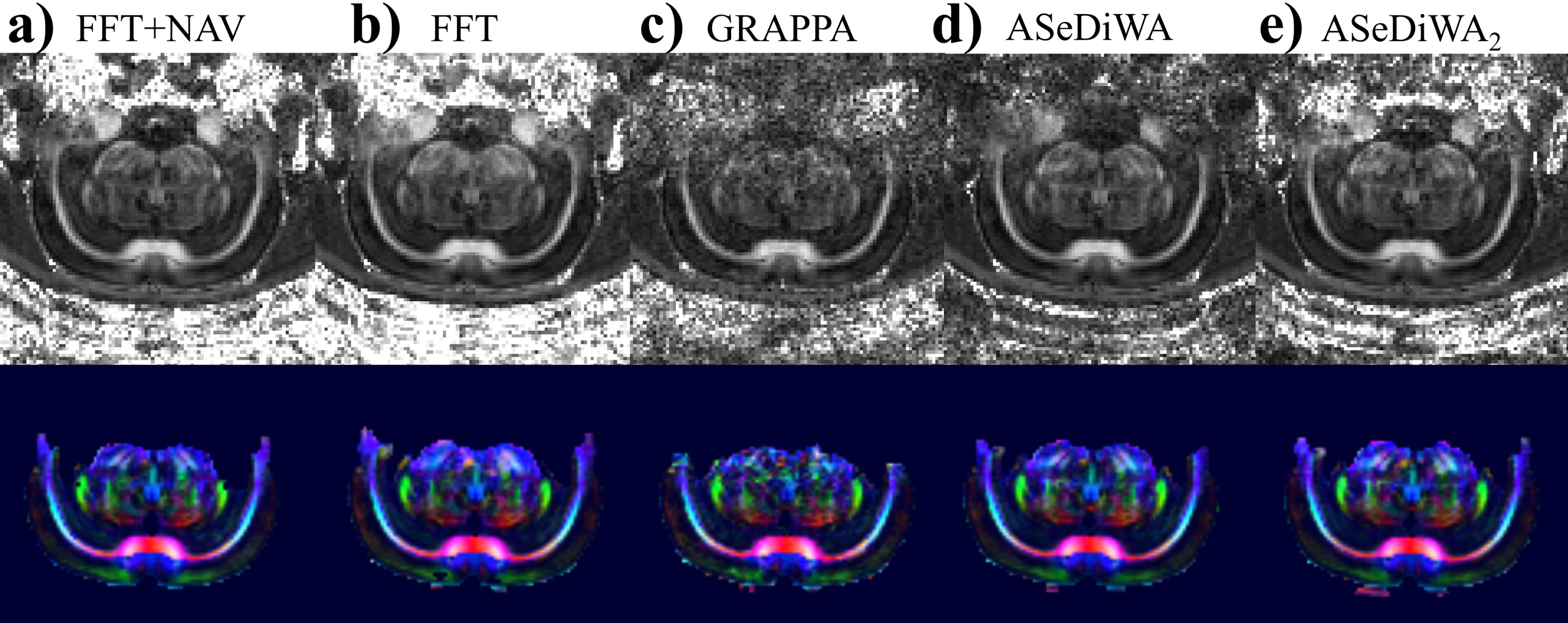
Figure 4: Fractional anisotropy and the corresponding color maps are shown for one
slice of the 4-channel rodent scan. a: navigator corrected reconstruction
(FFT). b: Standard (FFT) reconstruction without navigator correction. c:
separate GRAPPA reconstruction of each segment. d: ASeDiWA reconstruction
without further iterations, displaying improved SNR compared to the GRAPPA
result. e: ASeDiWA2 reconstruction with two additional iterations, further
improving reconstruction results.