1106
Assessment of Fatty liver disease in rats using quantitative transport mapping (QTM) method against pathology validation1Cornell University, New York, NY, United States, 2Weill Cornell Medical College, New York, NY, United States
Synopsis
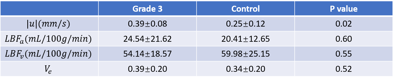
We propose to assess the severity of Nonalcoholic fatty liver disease (NAFLD) using quantitative transport mapping (QTM), a recently introduced flow quantification method. A numerical simulation was performed to compare QTM with traditional kinetic modeling. QTM successfully reconstructed blood flow with high accuracy (relative root mean square error = 0.27). Using DCE MRI in 5 adult rats with methionine choline-deficient diet-induced NAFLD (grade F3) and in 13 untreated control rats, only the QTM derived velocity |u| showed a significant difference between NAFLD and healthy controls.
Introduction
Nonalcoholic fatty liver disease (NAFLD) may cause different liver disease, including liver fibrosis, liver cirrhosis and nonalcoholic steatohepatitis1,2. Assessing NAFLD severity using dynamic contrast enhanced MRI (DCE-MRI) was proposed in a recent study which applied two-compartment kinetic modeling method3. Kinetic modeling is known to suffer from the delay and dispersion induced quantification errors, and depends on the choice of AIF. In this study, we propose to apply a recently developed flow quantification method, quantitative transport mapping (QTM)4, to NAFLD grading. We validate QTM in a vasculature flow simulation and compare its performance in NAFLD grading on a rat DCE-MRI dataset.Methods
QTM Algorithm: We use the transport equation to model the transport of tracers4:$$\partial _{t} c(\xi,t)=-\nabla\cdot c(\xi,t) u(\xi) \qquad (1)$$
where $$$c(\xi,t)$$$ is the tracer concentration in a voxel $$$\xi$$$,$$$\nabla$$$the spatial gradient, and $$$u(\xi)$$$ the average velocity in that voxel. Rewriting Eq.1 as $$$A\overrightarrow u = \overrightarrow b$$$ , where A is a large sparse matrix, $$$\overrightarrow u$$$ a large vector concatenating $$$u(\xi)$$$ for all voxels, and $$$\overrightarrow b$$$ a large vector concatenating $$$c(\xi,t)$$$ for all voxels and all time points. The inverse problem of reconstructing the velocity field $$$\overrightarrow u$$$ is formulated as a constrained minimization problem:
$$\overrightarrow u = argmin_{\overrightarrow u} ||A\overrightarrow u-\overrightarrow b||_{2}^{2}+\lambda||\nabla \overrightarrow u||_{1} \qquad (2)$$
An L1 regularization is added in Eq.2 for denoising with $$$\lambda=10^{-3}$$$ chosen empirically according to minimal mean square error with respect to the ground truth for the simulation and image quality and L-curve characteristics for the in vivo data.
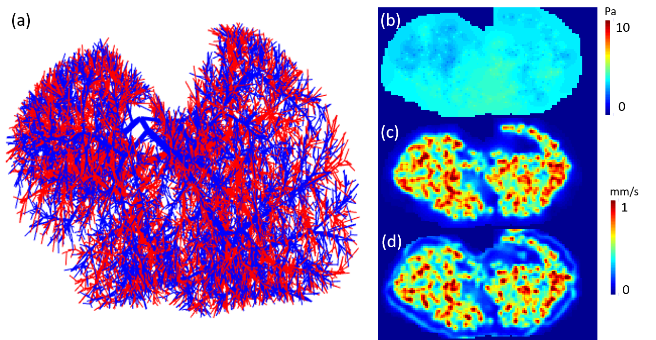
Numerical simulation: The vascular network acquired from a previous study5 is shown in Figure 1a, where the red segments represents the aorta and blue segments represents portal vein. The flow inside and outside the vessel network is simulated based on Poiseuille's law and Darcy’s law, respectively5. Tracer propagation is then simulated based on the transport equation. Simulated flow (shown in Figure 1c) and tracer concentration profile are then down-sampled to $$$[0.5,0.5,0.5] mm^3$$$, consistent with MRI imaging parameters (see below). QTM method is applied to the simulated tracer concentration profile and the reconstructed velocity map is compared with the ground truth velocity map.
In vivo DCE-MRI: 18 rat liver DCE-MRI scans (5 NAFLD grade3, 13 untreated control) were acquired using a T1-weighted 3D MRI sequence before and after the injection of gadolinium contrast agent using the following parameters: $$$[0.5,0.5,0.5] mm^3$$$ voxel size, 512x512x36 matrix, 5.6 s temporal resolution, and 60 time points. The DCE 4D image data was converted to gadolinium concentration ([Gd]) data by assuming a linear relationship between signal intensity change and contrast agent concentration6. QTM (Eq.2) was applied on the resulting concentration maps. The velocity amplitude of each voxel was calculated as:
$$|u(\xi)|=\sqrt {(u^x(\xi))^2+(u^y(\xi))^2+(u^z(\xi))^2} \qquad (3)$$
For comparison, the arterial blow flow ($$$LBF_a$$$ ), the portal venous blood flow ($$$LBF_v$$$ ), and the extravascular space volume ($$$V_e$$$) were computed based on a dual-input one compartment exchange model7:
$$\partial_t c(\xi,t)=LBF_a(\xi)c_a(t)+LBF_v(\xi)c_v(t)-\frac{(LBF_a(\xi)+LBF_v(\xi))}{V_e(\xi)}c(\xi,t) \qquad (4)$$
Here $$$c_a(t)$$$ and $$$c_v(t)$$$ are artery and portal vein input function, respectively. Statistical analysis was performed on the perfusion parameters averaged in a region of interest (ROI).
Results:
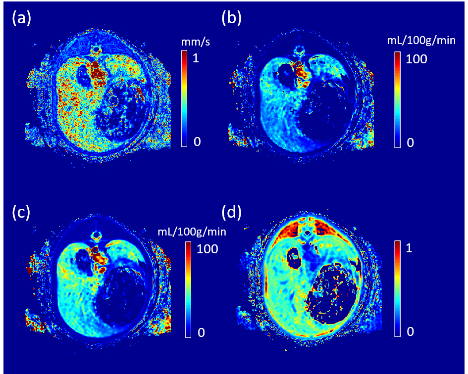
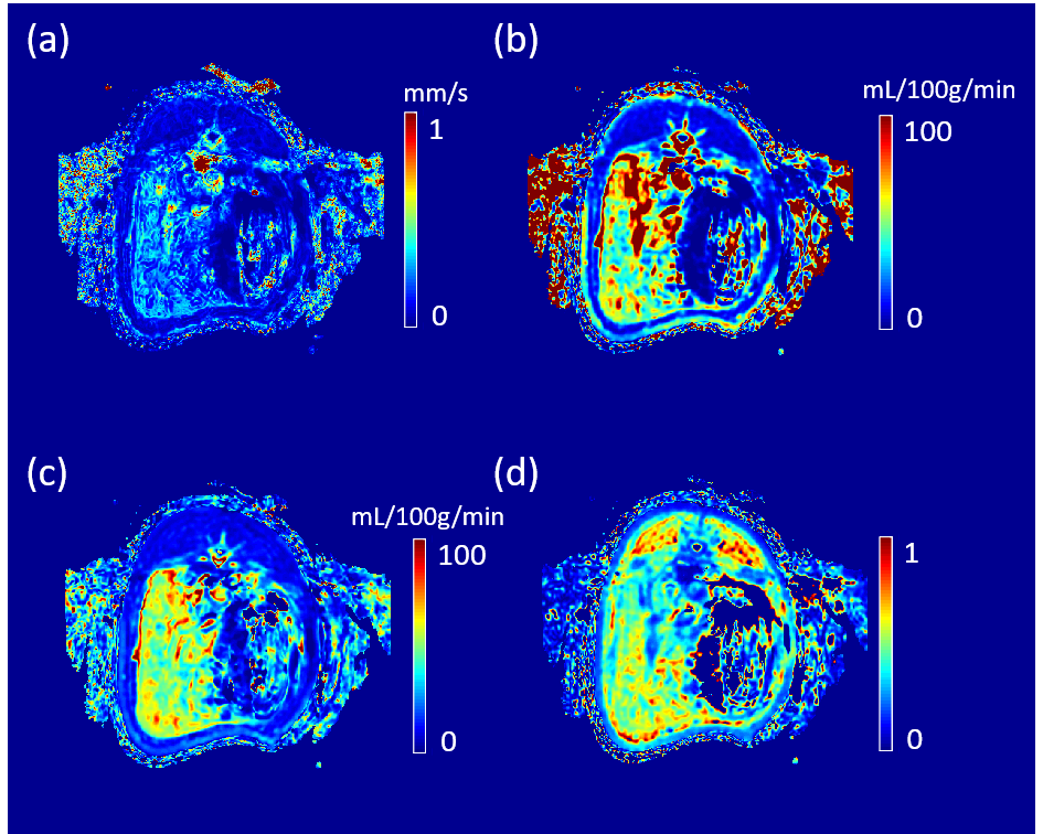
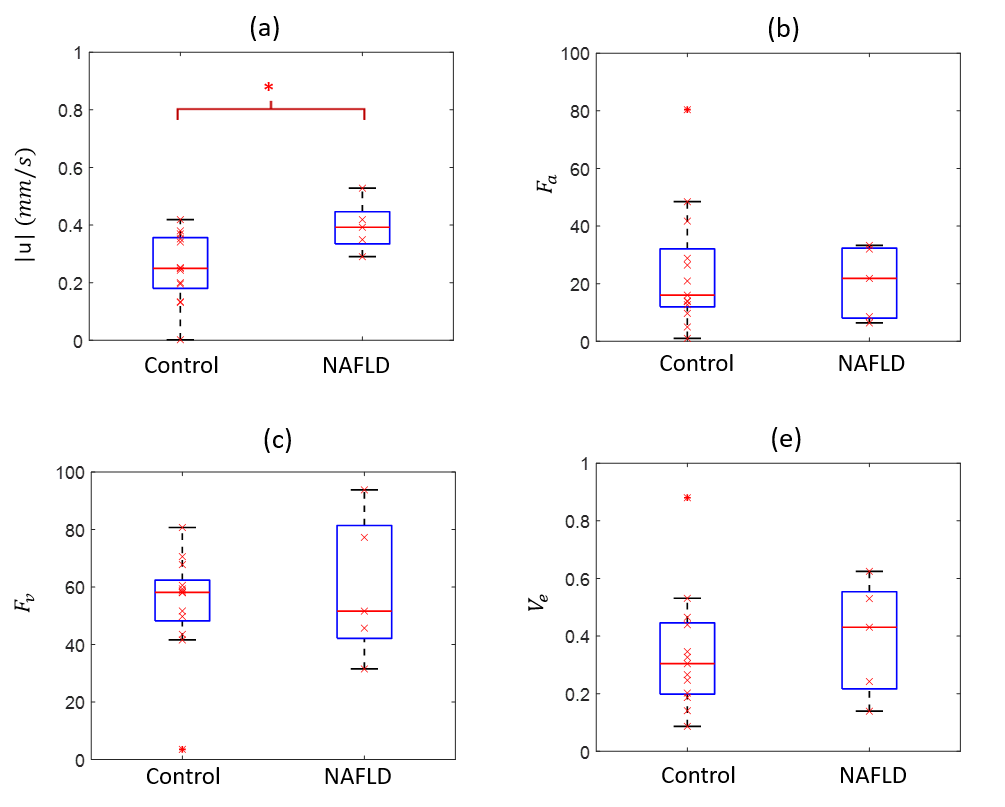
The reconstructed velocity from the simulated tracer concentration profile is shown in Figure 1d. Compared with the ground truth, QTM velocity showed good accuracy (rRMSE=0.27, linear regression $$$R^2$$$ =0.80). QTM velocity map,$$$LBF_a$$$ ,$$$LBF_v$$$ and $$$V_e$$$ map of a grade 3 NAFLD and a control case are shown in Figures 2 and 3, respectively. Only the QTM velocity showed a significant difference between NAFLD grade 3 and untreated control group (Figure 4 and 5).Discussion and Conclusion:
QTM can reconstruct the liver blood flow with good accuracy in a numerical simulation. Compared with kinetic modeling, QTM showed the highest diagnostic accuracy for assessing NAFLD based on DCE-MRI data. Future work may include adding compartment modeling to QTM and applying QTM in human NAFLD assessment.Acknowledgements
We don't have acknowledgements.References
1. Szczepaniak, Lidia S., et al. "Magnetic resonance spectroscopy to measure hepatic triglyceride content: prevalence of hepatic steatosis in the general population." American Journal of Physiology-Endocrinology and Metabolism 288.2 (2005): E462-E468.
2. Vernon G, Baranova A, Younossi Z M. Systematic review: the epidemiology and natural history of non‐alcoholic fatty liver disease and non‐alcoholic steatohepatitis in adults[J]. Alimentary pharmacology & therapeutics, 2011, 34(3): 274-285.
3. Wu Z, Cheng Z L, Yi Z L, et al. Assessment of Nonalcoholic Fatty Liver Disease in Rats Using Quantitative Dynamic Contrast‐Enhanced MRI[J]. Journal of Magnetic Resonance Imaging, 2017, 45(5): 1485-1493.
4. Bear J. Dynamics of fluids in porous media: Courier Corporation; 2013 4. Zhou L, Zhang Q, Spincemaille P, et al. Quantitative transport mapping (QTM) of the kidney with an approximate microvascular network[J]. Magnetic Resonance in Medicine, 2020.
5. Schwen L O, Krauss M, Niederalt C, et al. Spatio-temporal simulation of first pass drug perfusion in the liver[J]. PLoS Comput Biol, 2014, 10(3): e1003499.
6. Schabel MC, Parker DL. Uncertainty and bias in contrast concentration measurements using spoiled gradient echo pulse sequences. Phys Med Biol 2008;53(9):2345-2373.
7. Jafari R, Chhabra S, Prince M R, et al. Vastly accelerated linear least‐squares fitting with numerical optimization for dual‐input delay‐compensated quantitative liver perfusion mapping[J]. Magnetic resonance in medicine, 2018, 79(4): 2415-2421.
Figures