Introduction

The physics principle governing the passage of a tracer in tissue is the transport equation of mass flux¹. This transport equation based description of perfusion precludes the notion of arterial input function (AIF)². The inverse problem of the transport equation has recently been considered for mapping the 3D velocity field of water transit in tissue from multi-delay 3D arterial spin labeling MRI data^2,3, and is termed as quantitative transport mapping (QTM).
To access the transport of tracers that is permeable to the vessel wall, for example in dynamic contrast enhanced (DCE) MRI, an additional compartment corresponding to the extravascular space is needed for modeling in QTM, similar to traditional kinetic modeling. The tracer concentration in the extravascular space can be expressed using the total concentration in the voxel and the permeability of each voxel by integrating the exchange equation between two compartments, thus allowing the velocity and permeability to be solved based on the transport equation. This algorithm is validated in a porous media simulation and tested on rat DCE MRI data.

Methods

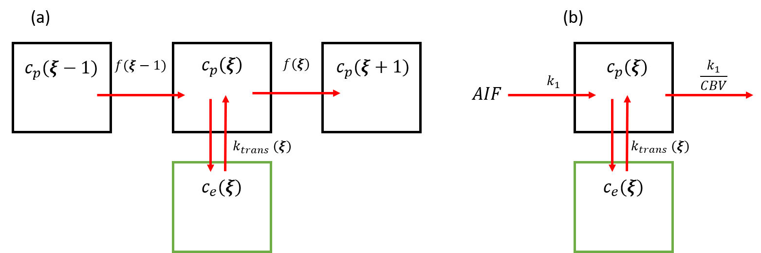
Two compartment QTM: Tracer amount change in vascular volume ( $$$V_p$$$ ) and extravascular space ($$$V_e$$$ ) can be expressed using the following equation:
$$ \partial _{t}V_pc_p(\xi,t)=-\nabla\cdot V_pc_p(\xi,t)\mathbf{f}(\xi)-k_{trans}(\xi)c_p(\xi,t)+k_{trans}(\xi)c_e(\xi,t) \qquad (1) $$
$$\partial _{t}V_ec_e(\xi,t)=k_{trans}(\xi)c_p(\xi,t)-k_{trans}(\xi)c_e(\xi,t) \qquad (2)$$
$$C(\xi,t)=V_pc_p(\xi,t)+V_ec_e(\xi,t) \qquad (3)$$
Here $$$C(\xi,t)$$$ is the tracer amount in the voxel , $$$c_p(\xi,t)$$$ and $$$c_e(\xi,t)$$$ are tracer concentration in vascular space and extra vascular space. $$$k_trans(\xi,t)$$$ is the exchange rate, $$$\mathbf{f}=[f^x,f^y,f^z]$$$ the averaged flow in three directions. Integrating Eq.2 with time, and replace $$$c_p$$$ in Eq.1 with $$$C$$$ using Eq.3, we get the following equation:
$$ \partial _{t}C(\xi,t)=-\nabla\cdot((c(\xi,t)-\frac{k_{trans}(\xi)}{V_p}e^{-k_{trans}(\xi)(\frac{1}{V_p}+\frac{1}{V_e})t}\int_{0}^{t}{c(\varepsilon)e^{k_{trans}(\varepsilon)(\frac{1}{V_p}+\frac{1}{V_e})\varepsilon}d\varepsilon })\mathbf{f}(\xi))\qquad (4) $$
Eq.4 is a nonlinear equation to $$$f$$$, $$$k_{trans}$$$,$$$V_e$$$ and $$$V_p$$$ . In this study, we consider a simpler situation that $$$V_e$$$ and $$$V_p$$$ are known. $$$f$$$ and $$$k_{trans}$$$ can then be solved from Eq.4 using Levenberg-Marquart method:
$$\mathbf{f}(\xi),k_{trans}(\xi)=argmin_{f,k_{trans}}\sum_{t=1,2,..N}||\partial_tc(\xi,t)+\nabla\cdot((c(\xi,t)-\frac{k_{trans}(\xi)}{V_p}e^{-k_{trans}(\xi)(\frac{1}{V_p}+\frac{1}{V_e})t}\int_{0}^{t}{c(\varepsilon)e^{k_{trans}(\varepsilon)(\frac{1}{V_p}+\frac{1}{V_e})\varepsilon}d\varepsilon })\mathbf{f}(\xi))||_2^2+\lambda_1||\nabla f||^1+\lambda_2||\nabla k_{trans}||^1 \qquad (5)$$

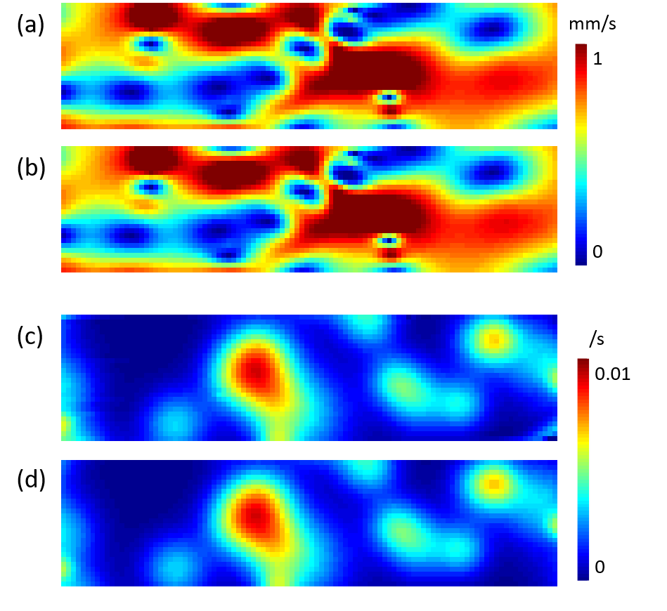
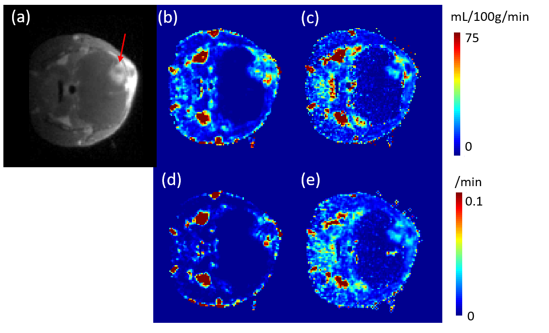
An L1 regularization is added in Eq.5 for denoising with $$$\lambda_1=10^{-4}$$$ and $$$\lambda_2=10^{-5}$$$ chosen empirically according to minimal mean square error with respect to the ground truth in simulation and in vivo image quality and L-curve characteristics. The flux rate in vascular space ($$$F$$$) can be calculated as follows: $$ F(\xi)=\sqrt{(f^x(\xi)^2+f^y(\xi)^2+f^z(\xi)^2)} \qquad (6) $$ Numerical validation: We validated the inversion algorithm using a 2-D rectangle-shaped porous media simulation. The permeability map and exchange rate map are set as a mixed gaussian distribution (shown in figure 1a and 1c), and the velocity map is calculated using Darcy’s law with a constant pressure boundary condition: The left side is set as inlet with pressure=100Pa and the right side is set as out let with pressure=0. The tracer concentration is calculated based on transport equation, with the concentration input $$$c(t)=te^{-t/10}$$$. $$$V_p$$$ is assumed to be 0.05 and $$$V_e$$$ is assumed to be 0.95 in this simulation. Velocity and exchange rate are then calculated based on simulated concentration profile and compared with the ground truth.In vivo DCE MRI data processing: 3 rats with head tumor were scanned on a GE 3T scanner with the following parameters: $$$[0.3,0.3,1] mm^3 $$$voxel size, 128x128x36 matrix, 5.6 s temporal resolution, and 120 time points. $$$f$$$ and $$$k_{trans}$$$ are calculated using QTM method based on Eq.1 to 6. $$$V_p=0.05$$$ and $$$V_e=0.95$$$ are used for QTM reconstruction. As a comparison, $$$f$$$ and $$$k_{trans}$$$ can be calculated using two compartment kinetic modeling:
$$ \partial _{t}V_pc_p(\xi,t)=F(\xi)c_a(t)-{F(\xi)}c_p(t)-k_{trans}c_p(\xi,t)+k_{trans}(\xi)c_e(\xi,t) \qquad (7) $$
$$ \partial _{t}V_ec_e(\xi,t)=k_{trans}c_p(\xi,t)-k_{trans}(\xi)c_e(\xi,t) \qquad (8)$$
$$C(\xi,t)=V_pc_p(\xi,t)+V_ec_e(\xi,t) \qquad (9)$$
$$$f$$$ and $$$k_{trans}$$$ can be solved from Eq.7-9 as a linear inversion problem. A L1TV regularization is added for inversion robustness and the regularization parameter $$$\lambda=10^{-3}$$$ is chosen based on L-curve study.

Results:

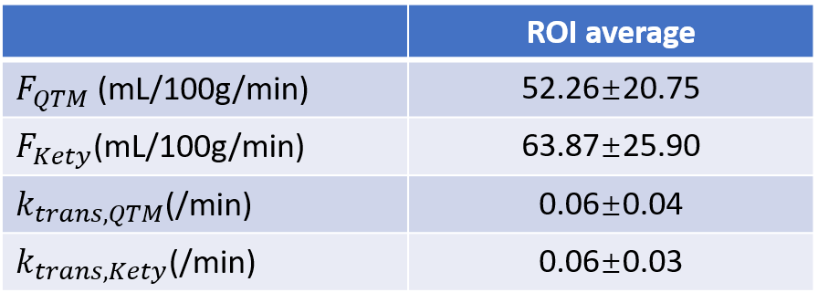
The two compartment QTM and two compartment kinetic modeling is illustrated in figure 1, where each black box represents a voxel, and each green box represents the corresponding extravascular space of the voxel. QTM method uses flow between neighboring voxels to represent transport in vascular space between voxels, while Kety's method uses arterial input function and a local decay function. Both QTM and kety's method use $$$k_{trans}$$$ to model tracer exchange between vascular and extravascular space.
In simulation, QTM method can reconstruct $$$F$$$ and $$$k_{trans}$$$ with high accuracy (rRMSE<0.01, figure 2b and 2d). $$$F$$$ and $$$k_{trans}$$$ calculated using QTM and kinetic modeling method of a rat brain tumor imaged using DCE MRI are shown in figure 3.

Discussion and Conclusion:

In this study, we extended QTM method with compartment modeling. The non linear inversion of QTM is validated on a porous media simulation. When applied to DCE MRI perfusion quantification, $$$f$$$ and $$$k_{trans}$$$ calculated using QTM method showed similar flow pattern, but no artery input function is needed. Further work may include applying 2c- QTM into perfusion quantification for patients and cross-validation of the calculated blood flow and tracer exchange rate with ASL and PET images.

Acknowledgements

We don't have any acknowledgements.