0909
Single echo reconstruction for rapid and silent MRI1Columbia MR Center, Columbia University, New York, NY, United States
Synopsis
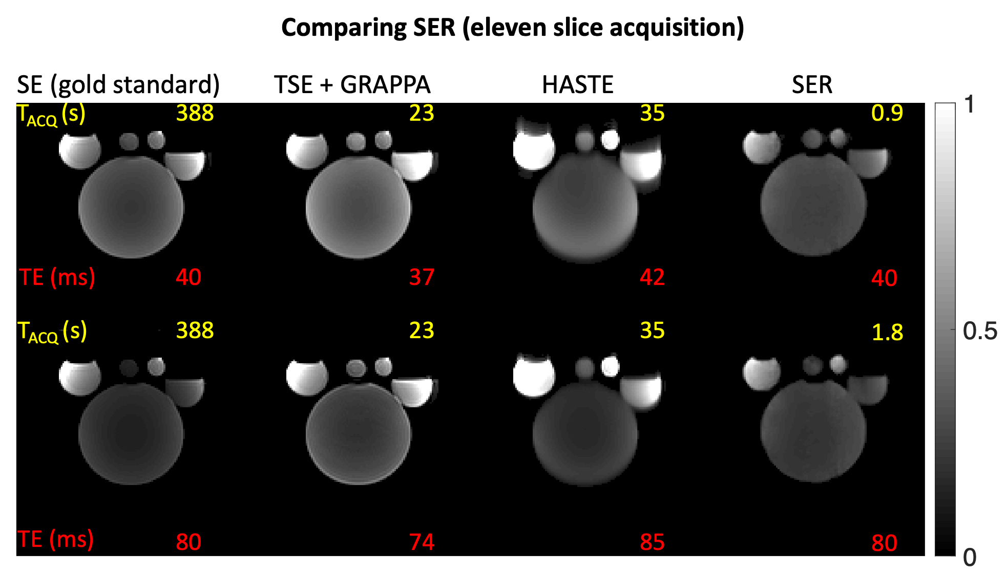
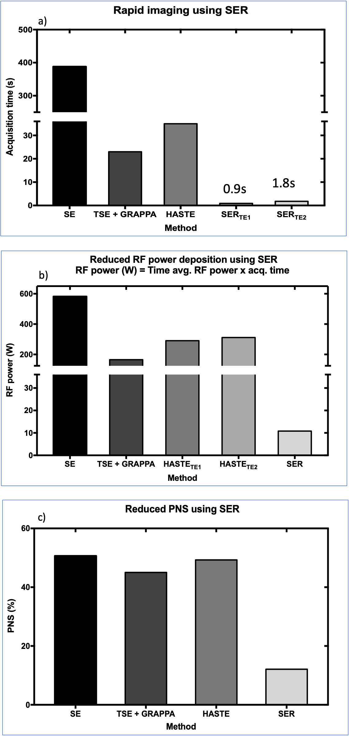
This work introduces a reconstruction-only approach, dubbed “single echo reconstruction” (SER) to demonstrate (i) the first, rapid 128 x 128 MRI without phase encoding using a 64-channel coil; (ii) significant reduction of RF power, PNS, and gradient noise; (iii) using only a commercially available coil with no external sensors (iv) comparison with gold-standard 2D spin-echo (SE) and accelerated acquisitions for $$$ T_2 $$$ weighted imaging as an application. For imaging 11 slices with TE = 80ms, the acquisition time was 1.8s with 10.8W total RF deposition, 12.09% peripheral nerve stimulation and no blurring artifacts.
Introduction
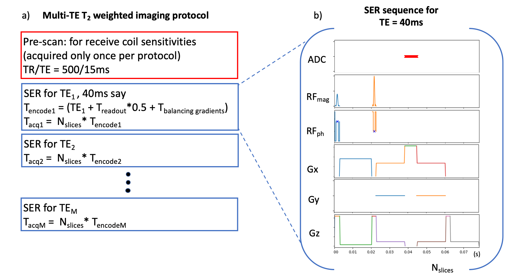
Acquisition time $$$ (T_{acq}) $$$ of a 2D MR image depends on repetition time $$$ (TR) $$$, number of views ($$$ N_v $$$ or phase encodes for Cartesian imaging), and number of signal averages $$$ (NSA) $$$ i.e. $$$ T_{acq} = TR* N_v *NSA $$$. Further, the acquisition speed is subject to radio-frequency (RF) power deposition, peripheral nerve stimulation (PNS), and gradient noise constraints. Reconstructing a 2D MR image from a single echo mitigates these multiple constraints. However, previous formulations (1, 2) and the associated study (2) using single echo acquisitions with a short Cartesian readout required the number of receive channels using stripline coils equal to $$$ N_v $$$ (2); or used external magnetosensors (3). In contrast, this work uses a reconstruction-only approach, dubbed “single echo reconstruction” (SER) to demonstrate (i) the first, rapid 128 x 128 MR imaging without phase encoding using a 64-channel coil, i.e., $$$ T_{acq} = T_{encode}*NSA $$$ where $$$ T_{encode} $$$ is the time to acquire one echo; (ii) significant reduction of RF power, PNS, and gradient noise; (iii) using only a commercially available coil with no external sensors (iv) comparison with gold-standard 2D spin-echo (SE) and accelerated acquisitions for $$$ T_2 $$$ weighted imaging as an application.Methods
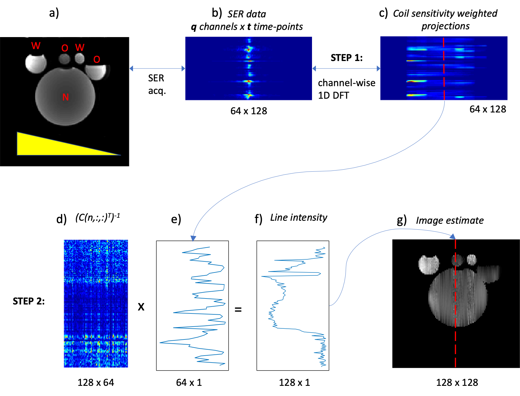
Acquisition: The gold standard (GS) method included a 2D multi-slice spin-echo (SE) acquired at two different echo times (TE = 40ms, 80ms). Accelerated sequences included turbo SE (TSE) with a GRAPPA factor of 6, an echo-train-length of 7 and, the half Fourier acquisition single-shot TSE (HASTE). The SER protocol and pulse sequence are shown in fig. 1. Briefly, the pypulseq coded (4,5) sequence acquires only one readout without phase encoding gradients. The reference scan was a pypulseq 2D SE multi-slice with TR/TE = 500/15ms. All acquisitions were acquired on an in vitro phantom (fig. 2) using a 64-channel head coil, had a field-of-view of 256 x 256mm2, slice thickness=5mm, and eleven slices. The GS, accelerated sequences, and SER were evaluated for acquisition time, total RF power deposited, PNS stimulation, and contrast compared to GS, by recording values from the vendor's user interface (UI).Reconstruction: The SER method illustrated in figs. 2,3 consists of three steps. Let S be the signal collected over time $$$ (t) $$$ and channels $$$ (q) $$$. Let $$$ M(x,y) $$$ be the object and $$$ C(x_l,y_n,q_o) $$$ be the coil sensitivity at the location $$$ (x_l,y_n) $$$ for channel $$$ q_o $$$. Then the signal S is given by:
$$S(q, t) = \int_{x,y} M(x,y) C(x,y,q) e^{-i2\pi k_x(t)x} dx \ dy \ [1]$$
Step 1 computes the 1D discrete Fourier transform of $$$ S $$$ to provide coil-sensitivity weighted projections $$$ p $$$. These projections are then concatenated (Eq. [2], fig. 2)
$$ p(q_1,k) = F(S(q_1,t)) \ [2a] $$
$$ P(q,k) = \begin{bmatrix} p(q_1,k)\\ p(q_2,k)\\ .\\ .\\ p(q_{64},k)\\ \end{bmatrix} \ [2b] $$
Step 2 computes the line-intensity profiles of the object's estimate $$$ \hat M(x,y) $$$ by inverting the coil sensitivities for a particular column for all rows and channels (eq. [3], fig. 2 – step 2)
$$ \hat m(x, y_n) = C_T^{-1}(x,y_n, q)P(q,k_n) \ \ |\ n= 0,1,..., N-1 \ [3a] $$
$$ \hat M(x,y) = \begin{bmatrix} \hat m(x, y_1) \ \hat m(x,y_2) \ … \ \hat m(x,y_{128}) \end{bmatrix}\ [3b] $$
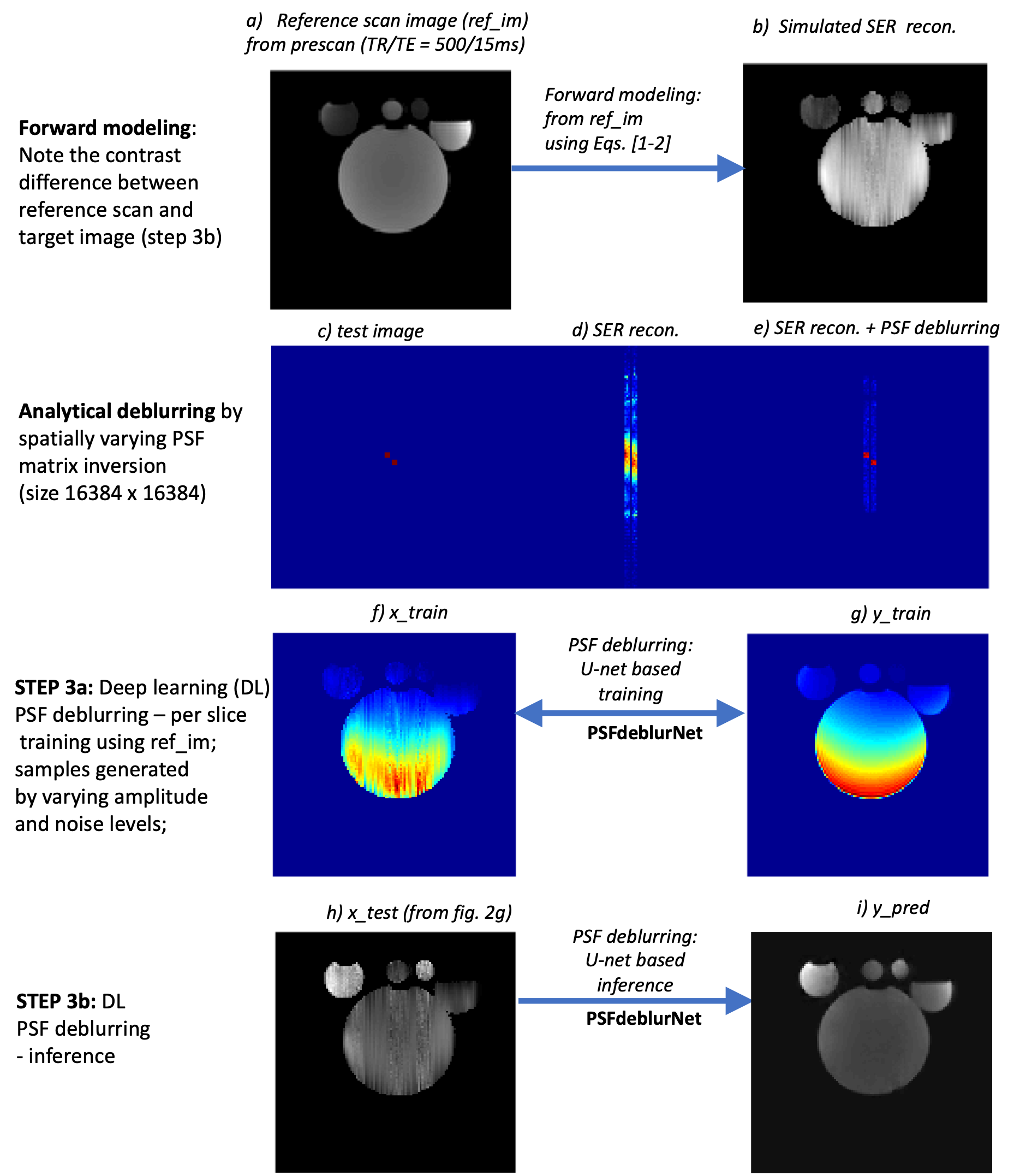
Step 2 represents an underdetermined system resulting in a spatially varying point spread function (PSF) blurring corrected in step 3 using a U-net (6) trained for 100 epochs, dubbed the PSFdeblurNet. This operation is analytically equivalent to characterizing the spatially varying PSF at each location and then inverting the entire PSF system matrix (fig. 3c-e). This inversion becomes untenable due to the large matrix size (16384 x 16384), leading to poor condition numbers. The deep learning equivalent PSFdeblurNet's training inputs are generated by forward-modeling the reference scan image using Eqs. [1-3] and corrupting the image by randomly varying amplitude and noise. Fig. 3 f,g shows an example of the training dataset. The models are trained per slice, and inferences are made on images from Eq.[3b] (see fig.3 h,i).
Results and Discussion
Fig. 4 shows the representative reconstructions of one of eleven slices at two TEs for all the methods considered. SER has similar contrast compared to GS without any blurring or saturation of intensities. Fig. 5 shows SER providing the i) highest acceleration (R=128), ii) least power deposited, and iii) the least PNS stimulation (also least gradient noise). In addition to the features in the introduction section, SER (i) does not require additional RF transmit channels for spatial encoding (fig. 1); (ii) does not suffer from blurring artifacts associated with multi-echo sequences (fig. 4); (iii) acceleration methods such as GRAPPA typically provide a reduction factor, $$$ R << N_v $$$ while SER achieves an $$$ R = N_v $$$ (figs. 1, 2, 5). SER requires a pre-scan to learn coil sensitivities similar to partial parallel imaging methods. The SER approach does not restrict its acquisition to any particular pulse sequence. This implementation is one of many possible pulse sequences and contrasts. Future work involves in vivo demonstration. SER can significantly accelerate multi-contrast imaging, improve temporal resolution, and enhance SNR through increased averaging.Acknowledgements
This work was supported and performed at the Zuckerman Mind Brain Behavior Institute MRI Platform, a shared resource, and Columbia MR Research Center site. The author would like to acknowledge funding from Zuckerman Institute Technical Development Grant for MR, CU-ZI-MR-T-0002; Zuckerman Institute Seed Grant for MR studies, CU-ZI-MR-S-0007
References
(1) Hutchinson M, Raff U. Fast MRI data acquisition using multiple detectors. Magnetic Resonance in Medicine 1988
(2) McDougall MP, Wright SM. 64-Channel array coil for single echo acquisition magnetic resonance imaging. Magnetic Resonance in Medicine 2005
(3) Lin FH, Wald LL, Ahlfors SP, Hämäläinen MS, Kwong KK, Belliveau JW. Dynamic magnetic resonance inverse imaging of human brain function. Magnetic Resonance in Medicine 2006
(4) Ravi, K.S., Potdar, S., Poojar, P., Reddy, A.K., Kroboth, S., Nielsen, J.F., Zaitsev, M., Venkatesan, R. and Geethanath, S., 2018. Pulseq-Graphical Programming Interface: Open source visual environment for prototyping pulse sequences and integrated magnetic resonance imaging algorithm development. Magnetic resonance imaging, 52, pp.9-15.
(5) Ravi, K.S., Geethanath, S. and Vaughan, J.T., 2019. PyPulseq: A Python Package for MRI Pulse Sequence Design. Journal of Open Source Software, 4(42), p.1725.
(6) Ronneberger, O., Fischer, P. and Brox, T., 2015, October. U-net: Convolutional networks for biomedical image segmentation. In International Conference on Medical image computing and computer-assisted intervention (pp. 234-241). Springer, Cham.
Figures