Introduction

MRI of short-T₂^* tissues such as bone, tendons, lung parenchyma, or teeth requires special short-TE pulse sequences such as UTE or ZTE. In ZTE the readout gradient is switched on before RF excitation, but finite RF pulse durations and hardware delays (i.e., dead time) result in a sampling gap at the center of k-space (1–4). The missing samples can be retrieved using single point imaging (SPI) in Cartesian space. In PETRA, the sampling gap increases with increasing spatial resolution, so that more SPI samples need to be acquired. As SPI is intrinsically time-inefficient, scan times in PETRA can become very long for high spatial resolutions or when long acquisition delays are used for quantitative imaging.
Compressed Sensing (CS) (5,6) has been used to drastically accelerate MRI data acquisitions. In this work, we apply CS to reduce the number of SPI samples in a PETRA sequence to enable sub-millimeter MRI of the knee in clinically acceptable measurement times.

Methods

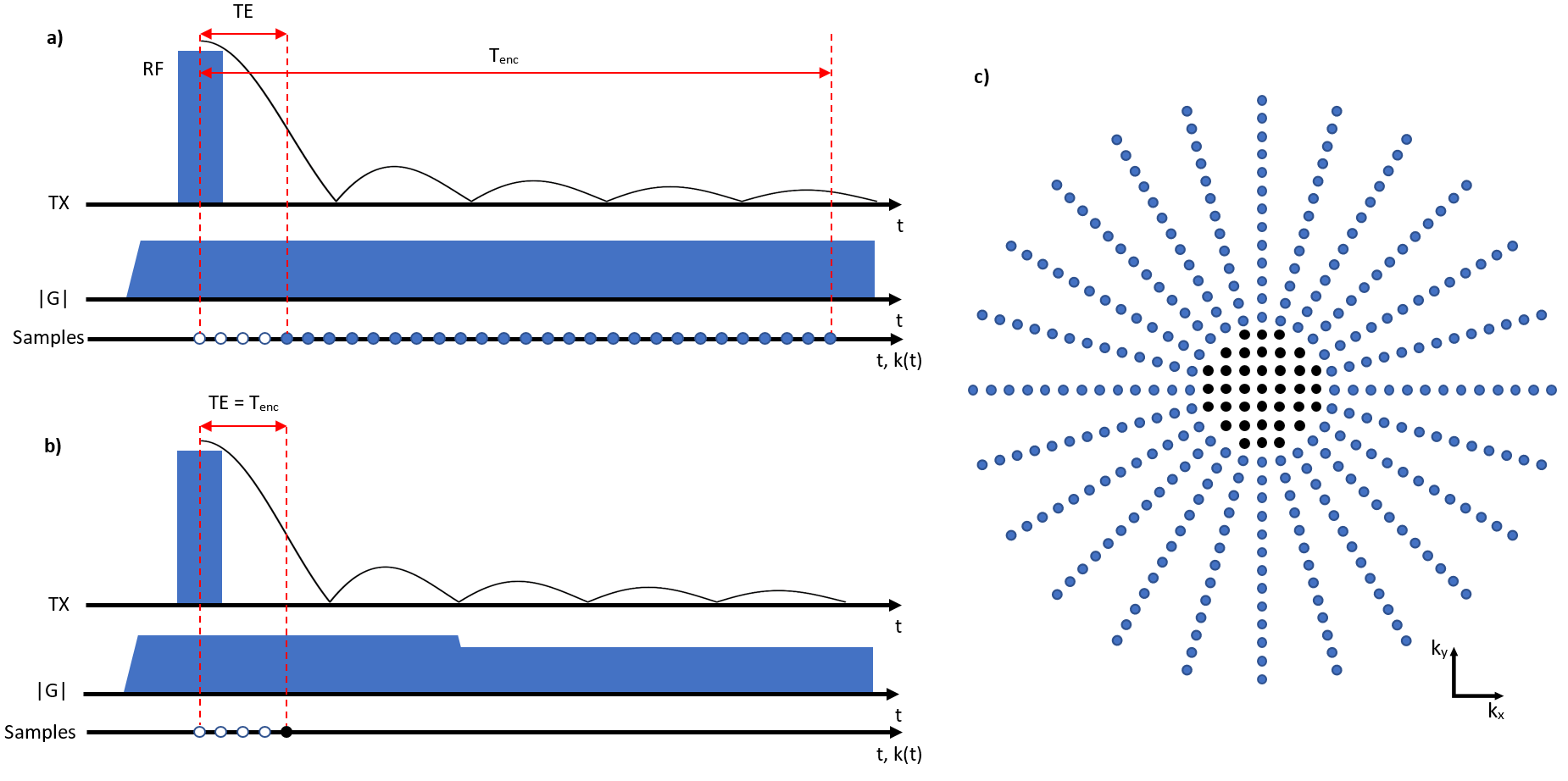
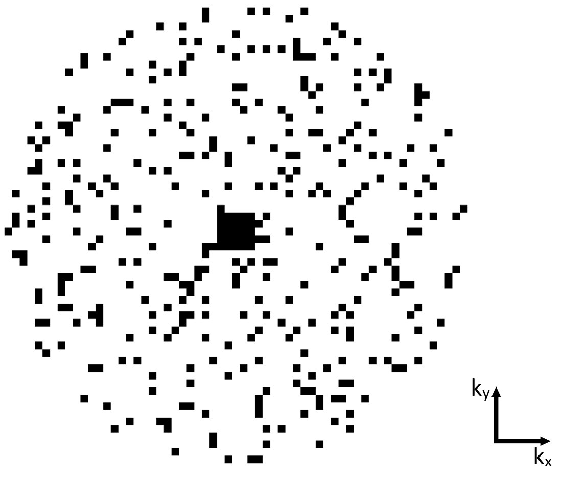
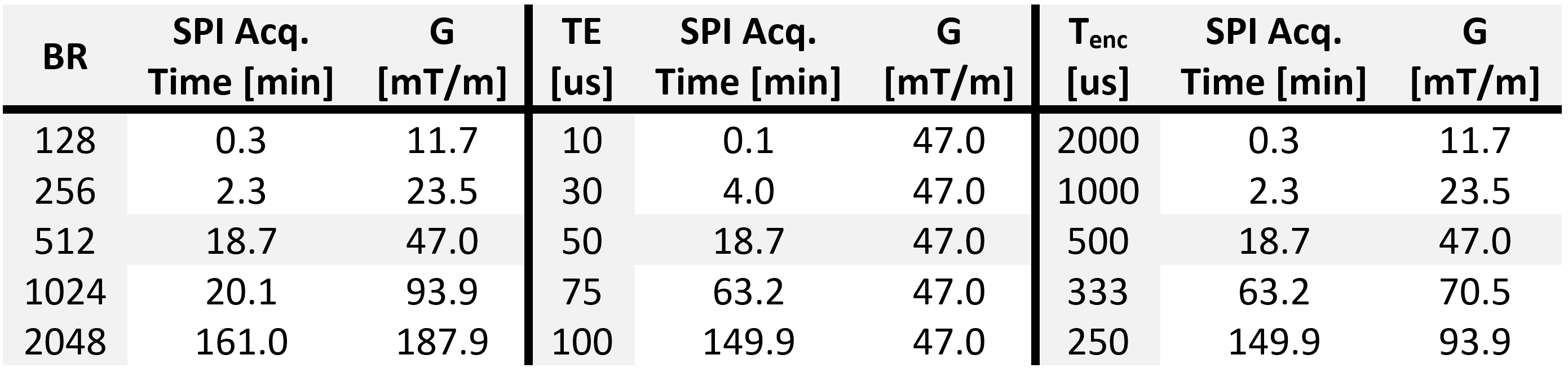
The PETRA sequence consists of a radial part where the required number of spokes in 3D is $$$N_\text{proj}=(\text{BR}\times\text{OS})^2\times\frac{\pi}{2}$$$ with the targeted base resolution $$$\text{BR}$$$, and an oversampling factor $$$\text{OS}$$$ (Fig. 1). As the center of k-space cannot be acquired directly, additional SPI data need to be sampled to fill the inner k-space. The k-space radius of the SPI section in PETRA is given by $$$N_\text{gap}=\frac{\text{TE}}{t_\text{dwell}}$$$, where $$$t_\text{dwell}$$$ is the dwell time. The required number of SPI samples is approximately $$$N_\text{spi}=\frac{4}{3}\pi(N_\text{gap})^3$$$. As $$$\frac{1}{t_\text{dwell}}=\text{BR}\times\text{OS}\times\frac{\text{BW}}{\text{pixel}}$$$, $$$N_\text{spi}$$$ has a cubic relation with $$$\text{BR}$$$, $$$\text{OS}$$$, $$$\text{BW/pixel}$$$ (or $$$\frac{1}{T_\text{enc}}$$$), and $$$\text{TE}$$$. In Table 1, measurement times for SPI acquisition w.r.t. $$$T_\text{enc}$$$, $$$\text{TE}$$$, and $$$\text{BR}$$$ are presented with the corresponding maximum gradient amplitude (|G|). Note that, for $$$\text{TE}$$$=50 µs, $$$\text{BR}$$$=512, $$$T_\text{enc}$$$=0.5 ms, and TR=2 ms, SPI acquisition time is more than 18 minutes.
To reduce the scan time for the SPI section, only a small portion of the SPI points is acquired in csPETRA. In Fig. 2 the sampling pattern for the SPI section at k_z=0 is presented. Essentially, near k-space center data are fully sampled over an inner k-space radius k_in, and a random sampling scheme is employed over the remaining SPI section. This choice of a sampling pattern was motivated by the need to maintain a high SNR, which is represented in the central k-space points.
For CS image reconstruction, the MR data was represented by a set of linear equations:$$\begin{bmatrix} s_1\\s_2\\\vdots\\s_C\end{bmatrix}=\begin{bmatrix} \mathcal{F}\Gamma_1\\\mathcal{F}\Gamma_2\\\vdots\\\mathcal{F}\Gamma_C\end{bmatrix}\mathbf{m}+\mathbf{n},$$$$\mathbf{s}=\mathbf{\mathcal{F}}\mathbf{m}+\mathbf{n},$$ where $$$s_c$$$ is the measured signal after regridding and density compensation by the $$$c$$$’th coil, $$$\mathcal{F}$$$ is the 3D discrete Fourier transform operator, $$$\Gamma_c$$$ is the sensitivity map of the $$$c$$$’th coil, $$$\mathbf{m}$$$ is the vectorized 3D image of the targeted object, and $$$\mathbf{n}$$$ is the noise. For the accelerated acquisition, the equation becomes: $$\mathbf{s}=\mathbf{M}\mathbf{\mathcal{F}}\mathbf{m}+\mathbf{n},$$ where $$$\mathbf{M}$$$ is the SPI sampling mask. As $$$\mathbf{M}$$$ is undersampled, the equation is in general ill-conditioned. So, we reconstructed the image by solving the following minimization problem: $$\underset{x}{\operatorname{argmax}} \lambda\text{TV}(\mathbf{m})+\alpha\|\mathbf{m}\|_1$$ $$\text{s.t.} \|\mathbf{M}\mathbf{\mathcal{F}}\mathbf{m}-\mathbf{s}\|_2<\epsilon,$$ where TV(⋅) is 3D total variation operator, $$$\|\cdot\|_1$$$ is $$$\ell_1$$$-norm operator, $$$\|\cdot\|_2$$$ is $$$\ell_2$$$-norm operator, $$$\lambda$$$ and $$$\alpha$$$ are scalar weights of TV and $$$\ell_1$$$-norm regularization operators, respectively. $$$\epsilon$$$ is the bound on the data fidelity error. $$$\ell_1$$$-norm and TV functions are selected as regularization terms.
The CS reconstruction was implemented using Alternating Direction Method of Multipliers (7) of the BART toolbox (8). The performance of the proposed approach was evaluated by measuring the root-mean-square-error (RMSE) level=$$$\sqrt{\frac{1}{N}\sum^N_{n=1}|\Delta_n|^2}$$$, where $$$\Delta$$$ is the difference image and $$$N=\text{BR}^3$$$ is the total number of voxels.
Experiments were performed on a 3T MRI system (MAGNETOM Prisma, Siemens, Erlangen, Germany) with a 15-channel TX/RX knee coil (QED, Cleveland, OH). In-vivo PETRA data of the knee of a healthy volunteer were acquired with a full SPI section: FOV = (20 cm)³, TR=2ms, $$$\text{TE}$$$=54µs, τ_RFpulse=8µs, α=5°, $$$t_\text{dwell}$$$ =2µs, voxel size = (0.5 mm)³, projections: 100,000, SPI points: 124,487, T_acq=7.5 mins. Undersampling with SPI was retrospectively applied – here, an acceleration rate (Acc) was defined as the total number of SPI points over the undersampled number.

Results

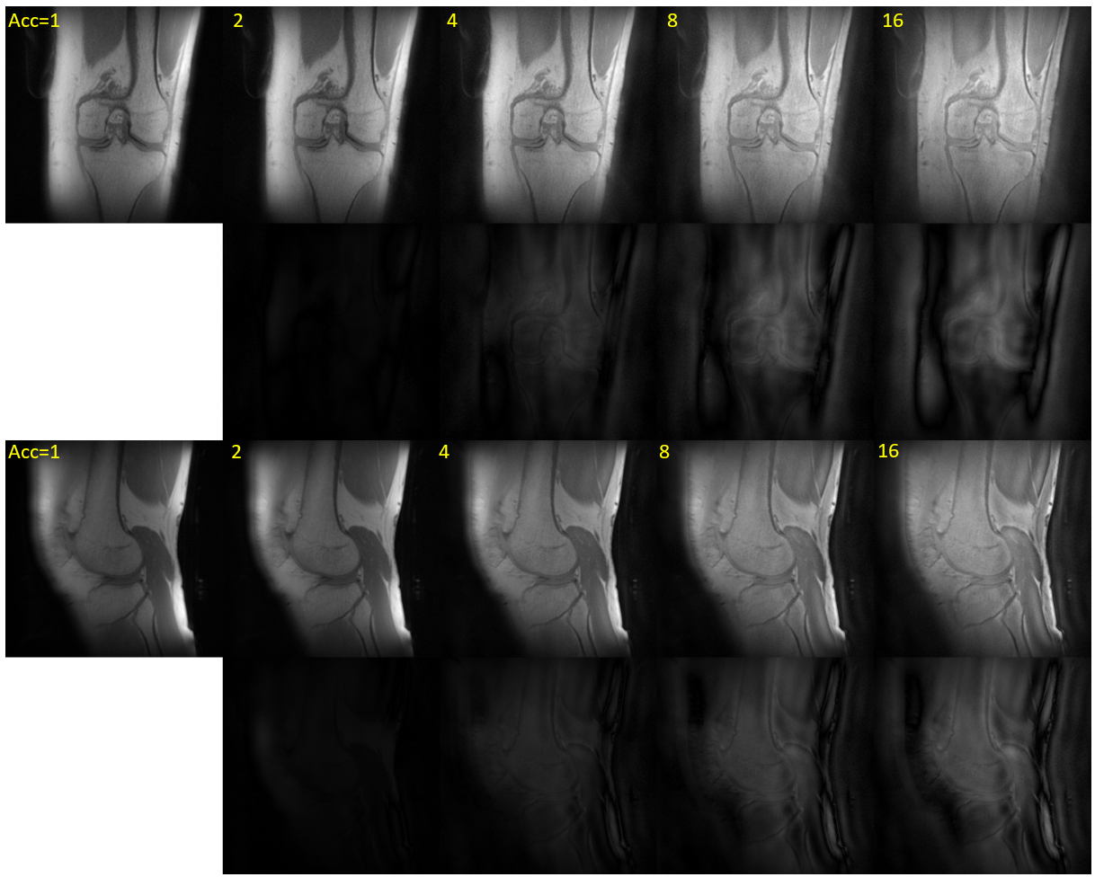
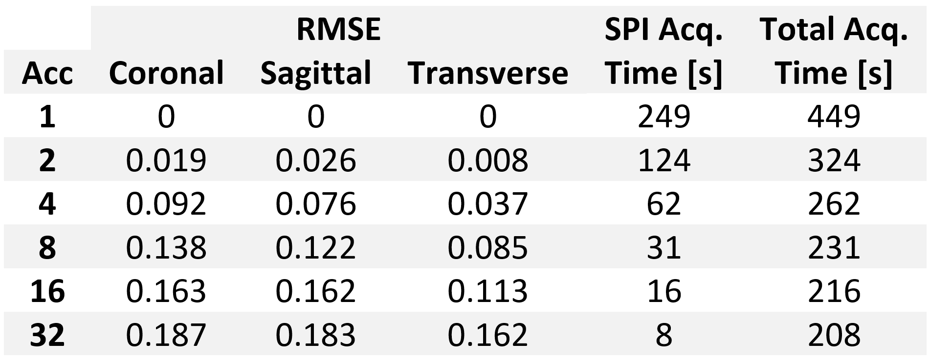
In Figure 3, in-vivo knee images acquired with PETRA (Acc=1) and csPETRA (Acc=2, 4, 8, and 16) are presented, together with the difference images below in the same windowing. Despite the undersampling, tendons, ligaments and menisci are clearly identified in both sagittal and coronal slices. RMSE for csPETRA images with Acc>1 is compared to the reference image (Acc=1). Table 2 shows the RMSE table of each image with its acquisition time. The RMSE is less than 10% (100xRMSE) up to Acc=4.

Discussion

csPETRA reduces the acquisition times significantly while preserving the anatomical details. The RMSE error was less than 10% up to a four-fold acceleration. To improve the image quality further, the undersampling mask can be optimized for targeted tissue and acceleration rates. The size of the fully acquired central k-space region can also be optimized. Reconstruction parameters (e.g., $$$\lambda$$$, $$$\alpha$$$, and $$$\epsilon$$$) can be adjusted based on SNR, sparsity, or other image features (9).
PETRA acquisitions are extremely long for TE values above a millisecond, since the time required for SPI acquisition increases dramatically. The proposed approach allows PETRA technique to be used in quantitative MRI applications, such as T₂^* mapping.

Acknowledgements

.