0904

Spectro-Dynamic MRI: Characterizing Bio-Mechanical Systems on a Millisecond Scale

Max H. C. van Riel^1,2, Niek R. F. Huttinga¹, and Alessandro Sbrizzi¹
¹Department of Radiotherapy, Computational Imaging Group for MR diagnostics and therapy, UMC Utrecht, Utrecht, Netherlands, ²Department of Biomedical Engineering, Medical Image Analysis, Eindhoven University of Technology, Eindhoven, Netherlands

Synopsis

Measuring in vivo dynamics can yield valuable information about the cardiovascular or musculoskeletal system. MRI shows severe limitations when dealing with motion at high spatial and temporal resolutions. We propose spectro-dynamic MRI for the characterization of dynamics directly from k-space data. The sampling pattern is adjusted to achieve a temporal resolution of a few milliseconds. A measurement model, relating the measured data to the displacements, is combined with a dynamical model, introducing prior knowledge about the dynamics. Preliminary results show that spectro-dynamic MRI allows estimation of motion fields and dynamical system parameters from heavily undersampled data on a millisecond timescale.

Introduction

Dynamic information can be valuable for the diagnosis and understanding of diseases in the cardiac¹ and musculoskeletal² systems. However, acquiring 3D MR images at a high spatial and temporal resolution simultaneously is challenging. Typical dynamic MRI techniques accelerate data acquisition by assuming a periodic motion of the heart, which is problematic for patients with arrhythmia.
Here we present spectro-dynamic MRI as a method to probe time-resolved dynamic information from spectral MRI data. A measurement model is combined with a dynamical model, which provides prior knowledge about the dynamics. The motion fields as well as the dynamical system parameters (e.g. myocardial stiffness) can be reconstructed. Both models take the form of partial differential equations with spatial and temporal derivatives. These derivatives can be calculated directly from heavily undersampled k-space data at a time interval of just a few milliseconds by using a properly tailored sampling pattern.

Theory

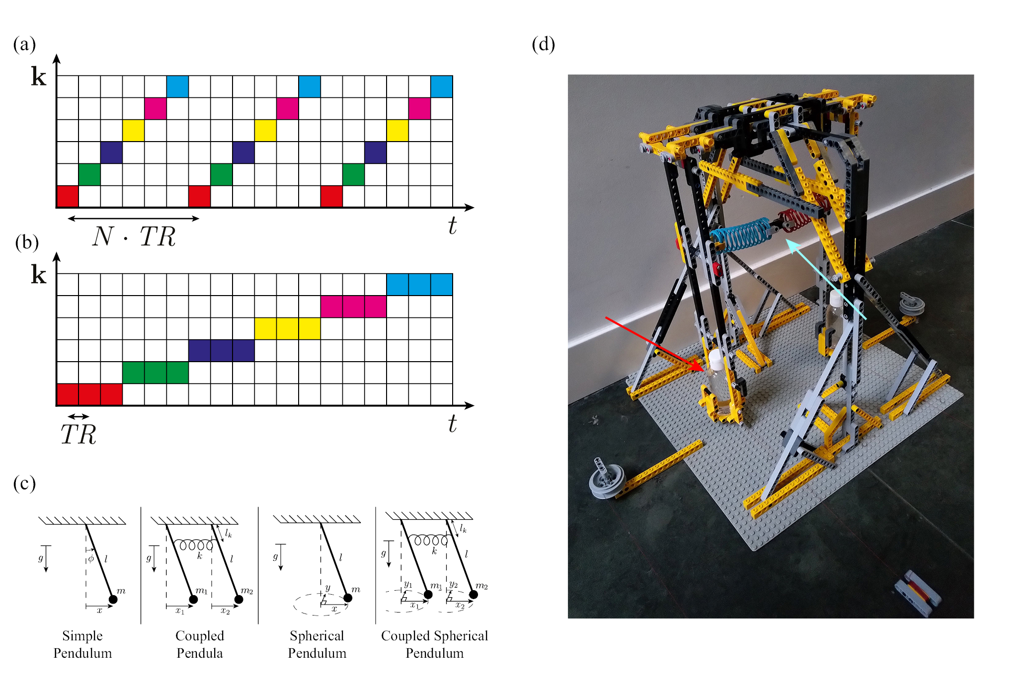
The temporal derivatives in both models can be estimated using finite differences. Doing this in the image domain leads to time steps in the order of seconds, since a fully sampled k-space is required for every image (Fig. 1(a)). In contrast, it is possible to acquire data in k-space at a temporal resolution in the order of milliseconds (Fig. 1(b)), thereby enabling the accurate computation of derivatives.
The measurement model $$$G$$$ relates the displacements $$$\mathbf{u}$$$ to the measured k-space data $$$M$$$ at spatial frequency $$$\mathbf{k}$$$ and time $$$t$$$: $$G(\mathbf{u},M,\mathbf{k},t)=0.$$Deriving this model using the conservation of the total magnetization results in:$$ G(\mathbf{u},M,\mathbf{k},t)=\frac{\partial}{{\partial}t}M(\mathbf{k},t)+i2\pi\sum_{j=1}^dk_jM(\mathbf{k},t)*\frac{\partial}{{\partial}t}U_j(\mathbf{k},t)+i2\pi\sum_{j=1}^dM(\mathbf{k},t)*k_j\frac{\partial}{{\partial}t}U_j(\mathbf{k},t)=0,$$where $$$U_j$$$ is the spatial Fourier Transform of the displacement field in the $$$j^\textrm{th}$$$ dimension, and the summations are taken over all $$$d$$$ spatial dimensions. Since the data is heavily undersampled to obtain motion fields at a high temporal resolution, a dynamical model $$$F$$$ is added, providing prior knowledge about the dynamics of the system:$$F(\mathbf{u},\boldsymbol{\theta},\mathbf{k},t)=0.$$This dynamical model contains a set of dynamical parameters $$$\boldsymbol{\theta}$$$. These are estimated next to the displacements by solving an optimization problem, where the dynamical model is used as a regularizer on the measurement model³:$$\min_{\mathbf{u},\boldsymbol{\theta}}\|G(\mathbf{u},M,\mathbf{k},t)\|_2^2+\lambda\|F(\mathbf{u},\boldsymbol{\theta},\mathbf{k},t)\|_2^2.$$

Methods

We performed several experiments with four different dynamical systems, see Fig. 1(c). A setup consisting of two pendula was made using LEGO, see Fig. 1(d). The pendula could swing in two directions and could be coupled together with a plastic spring. The dynamical model of all four systems can be described by a second order differential equation using a mass matrix $$$M_D(\boldsymbol{\theta})$$$ and a stiffness matrix $$$K_D(\boldsymbol{\theta})$$$, which depend on the dynamical parameters $$$\boldsymbol{\theta}$$$:$$M_D(\boldsymbol{\theta})\frac{d^2}{dt^2}\mathbf{u}(t)+K_D(\boldsymbol{\theta})\mathbf{u}(t)=\mathbf{0}.$$
The experiments were performed with a 1.5T MRI scanner (Ingenia, Philips Healthcare). Cartesian data acquisition in the coronal plane was performed with a spoiled gradient echo sequence (TR/TE = 4.4/2.1 ms, FA=9$$$^\circ$$$). Every readout line was repeated $$$N_\textrm{rep}$$$ times before moving on to the next line, as in Fig. 1(b). Reconstruction was done in Matlab (The MathWorks Inc.).
The estimated displacements in the readout direction were validated against a reference line. The natural frequencies of the dynamical systems, calculated using the estimated dynamical parameters $$$\boldsymbol{\theta}$$$, were compared to the frequency spectrum of this reference data. Additional undersampling was added retrospectively to investigate the behavior of the reconstructions with even fewer available data, down to only 2 datapoints for each readout.

Results

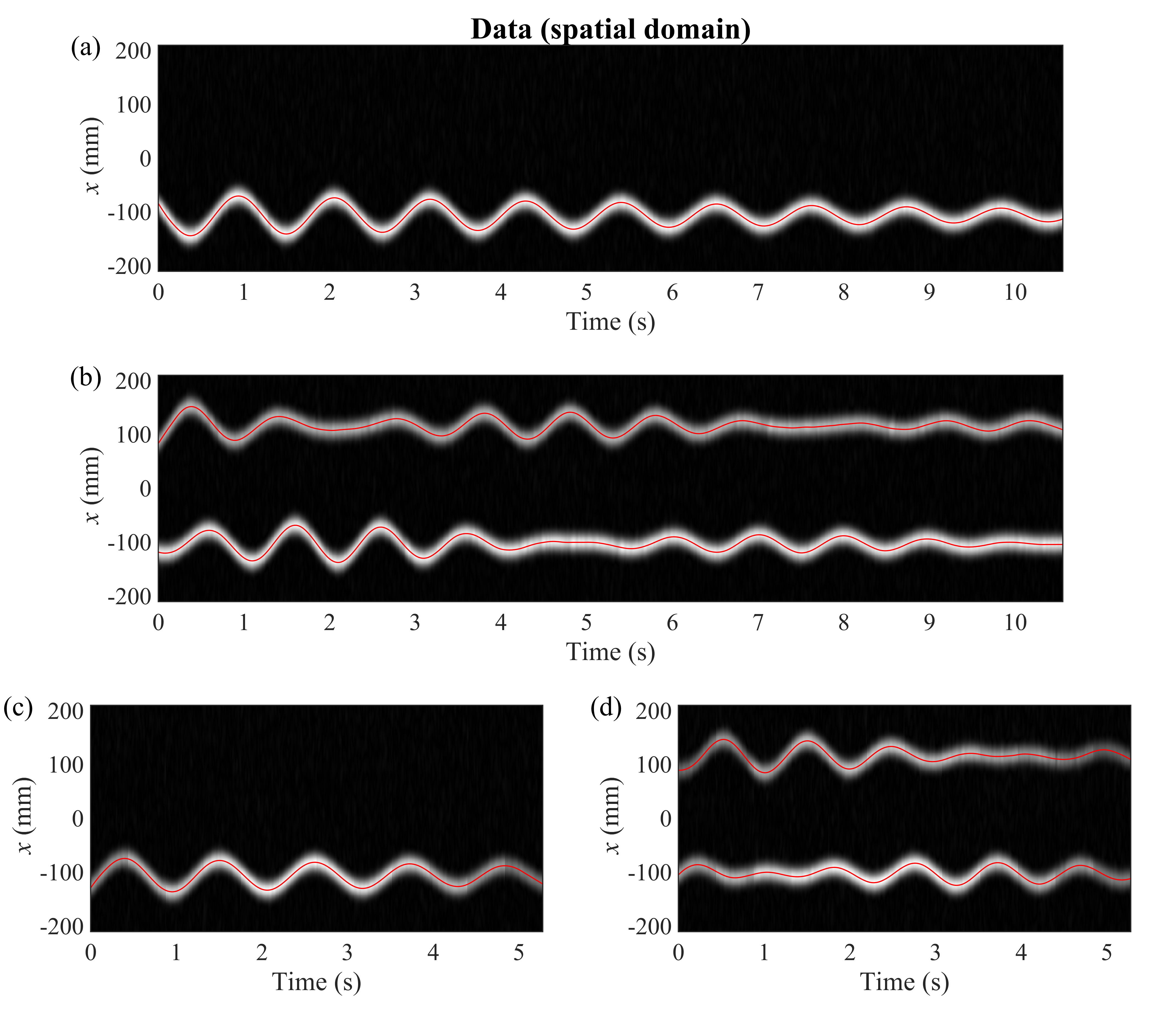
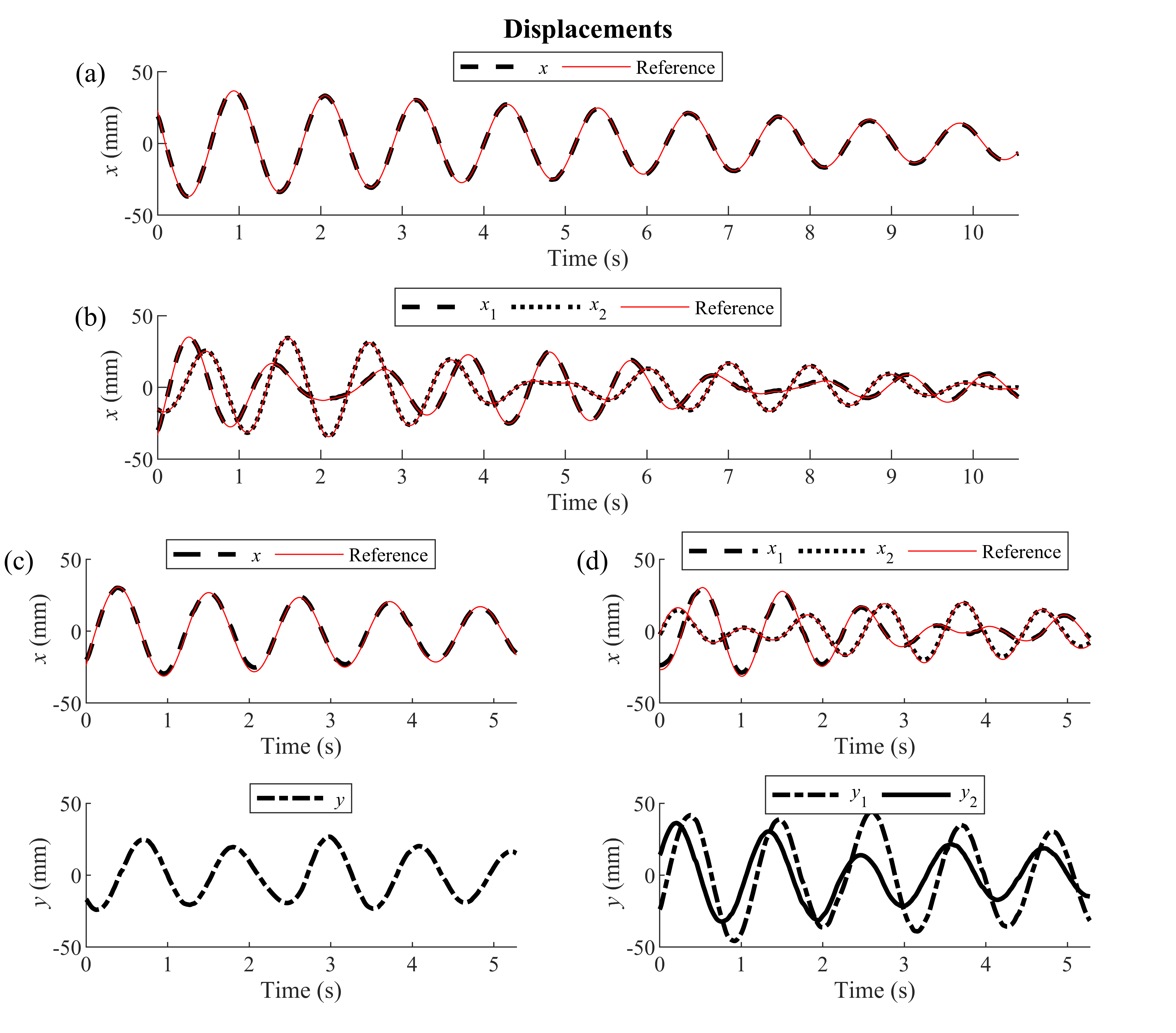
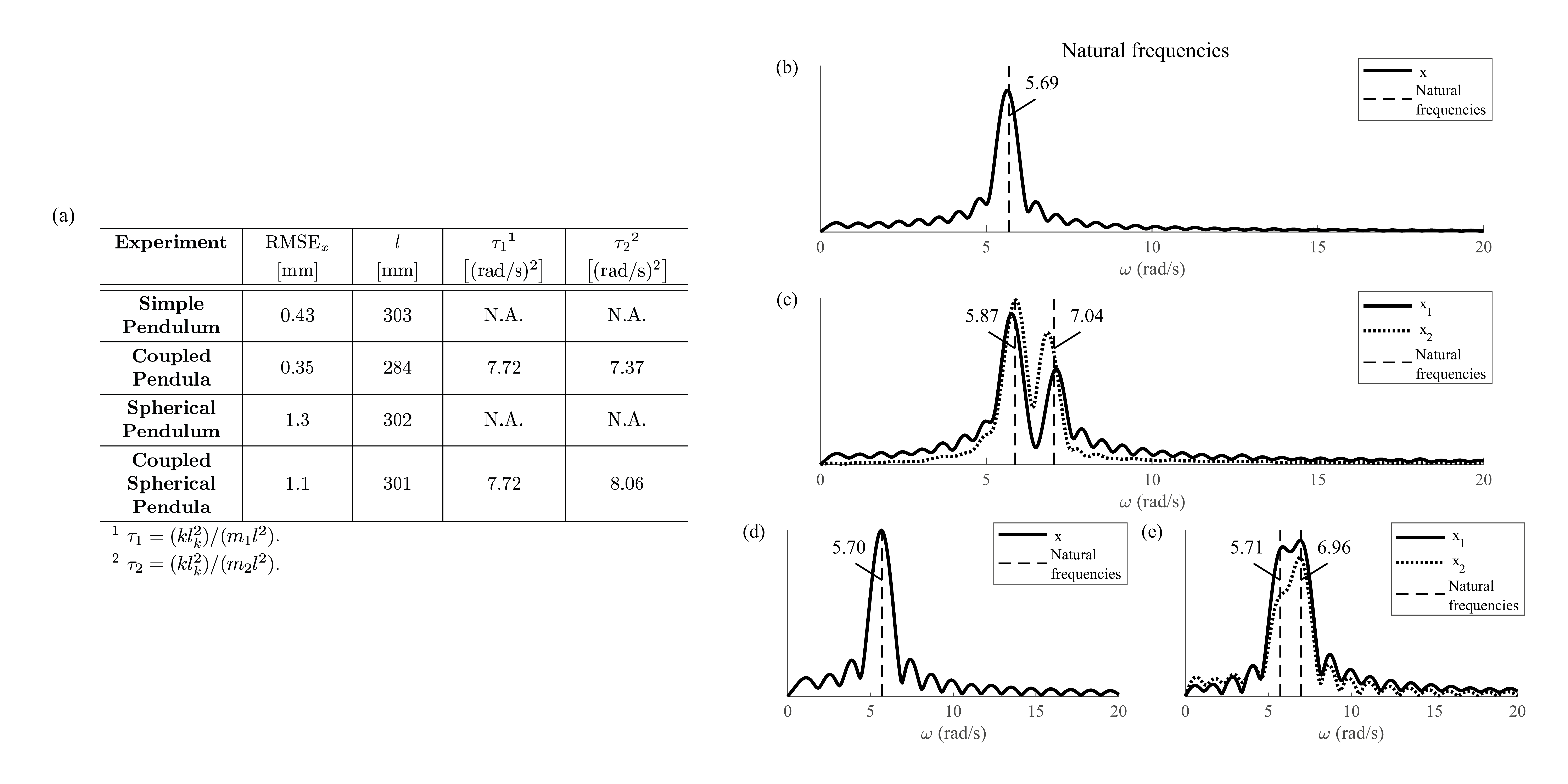
Fig. 2 shows the 1D FFT of every readout line. The data could only be visualized in the readout direction, as only a single phase encode index was sampled every readout. The (coupled) oscillations are clearly visible in this data. Additionally, this data was used to get the reference displacements.
The reconstructed displacements are shown in Fig. 3. The accuracy of the estimates, as well as the estimated dynamical parameters, can be seen in Fig. 4(a). The validation of $$$\boldsymbol{\theta}$$$ is shown in Fig. 4(b).
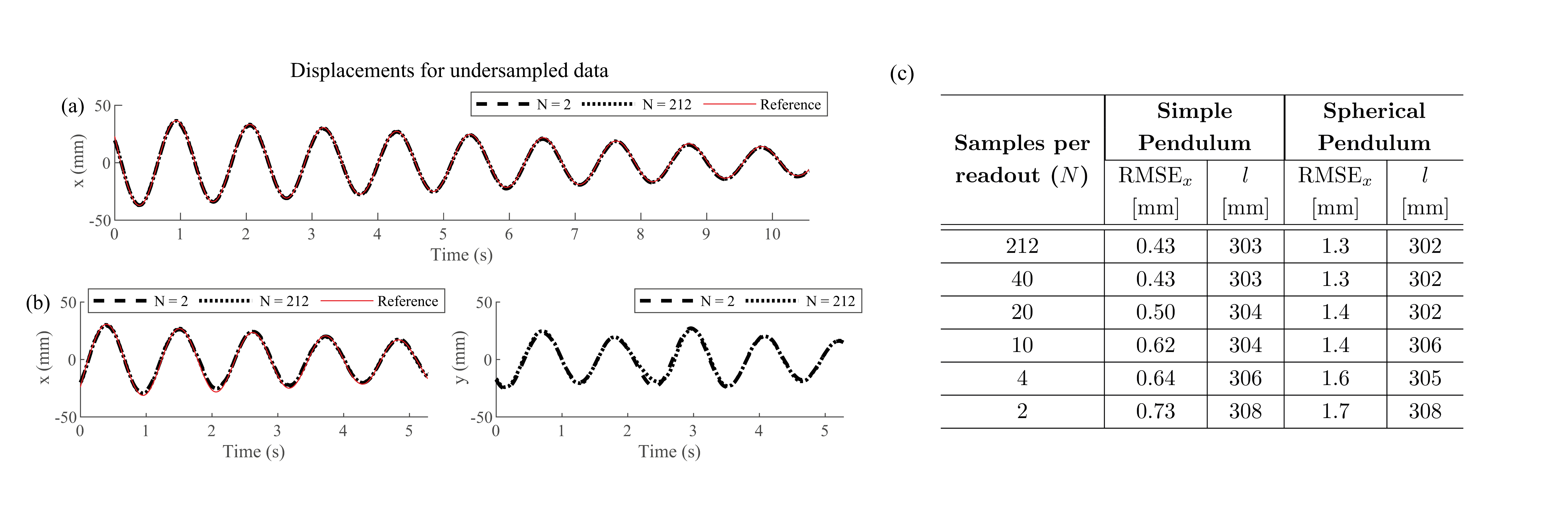
Fig. 5 shows the estimated displacements with the retrospectively undersampled data. The dynamics can still be estimated with only 2 sample points per readout, albeit with a slightly larger error.

Discussion

The estimated displacements in Fig. 3 correspond well to the reference displacements. Note that despite the absence of a friction term in the dynamical model, the decreasing amplitude of the motion could still be reconstructed.
The sampling pattern could be optimized further. Non-Cartesian sampling patterns, or an interleaved sampling pattern, could prove to be more beneficial. Further possible extensions of spectro-dynamic MRI are the reconstruction of 3D and non-rigid motion fields.
To measure in vivo dynamics, the dynamics of organ tissues must be modelled. Deriving these models by starting from first principles leads to very complex models with many parameters⁴. Data-driven discovery of dynamical systems^5–7 could provide phenomenological models with reduced complexity, while still capturing the intricate dynamics. In future work, these models could serve as dynamical model in the spectro-dynamic MRI framework.

Conclusion

We have presented spectro-dynamic MRI, a method that allows for characterization of dynamical systems at a temporal resolution of a few milliseconds. By combining a measurement model and a dynamical model, the displacement fields and the dynamical parameters of the system could be accurately estimated directly from k-space data, even with very high undersampling factors. The results are promising for potential future applications in the diagnosis of cardiac or musculoskeletal diseases.

Acknowledgements

We would like to thank professor Nico van den Berg and Tom Bruijnen for their help and advice regarding the execution of the experiments and the analysis of the data.

References

1. Amzulescu MS, De Craene M, Langet H, et al. Myocardial strain imaging: Review of general principles, validation, and sources of discrepancies. Eur Heart J Cardiovasc Imaging. 2019;20(6):605-619. doi:10.1093/ehjci/jez041

2. Shapiro LM, Gold GE. MRI of weight bearing and movement. Osteoarthr Cartil. 2012;20(2):69-78. doi:10.1016/j.joca.2011.11.003

3. van Leeuwen T, Herrmann FJ. A penalty method for PDE-constrained optimization in inverse problems. Inverse Probl. 2016;32(1):1-26. doi:10.1088/0266-5611/32/1/015007

4. Sermesant M. When Cardiac Biophysics Meets Groupwise Statistics: Complementary Modelling Approaches for Complementary Modelling Approaches for Patient-Specific Medicine. Signal and Image processing. Université de Nice - Sophia Anitpolis; 2016.

5. Daniels BC, Nemenman I. Automated adaptive inference of phenomenological dynamical models. Nat Commun. 2015;6:1-8. doi:10.1038/ncomms9133

6. Brunton SL, Kutz JN. Data-Driven Science and Engineering. Cambridge University Press; 2019. doi:10.1017/9781108380690

7. Rudy SH, Kutz JN, Brunton SL. Deep learning of dynamics and signal-noise decomposition with time-stepping constraints. J Comput Phys. 2019;396:483-506. doi:10.1016/j.jcp.2019.06.056

Figures

Figure 1: (a) In conventional MRI, a different line in k-space is sampled every repetition. (b) In spectro-dynamic MRI, one k-space line is repeated $$$N_\textrm{rep}$$$ times, reducing the time interval between the acquisition of the same data point in k-space. (c) Schematic representations of the four dynamical systems used for our experiments. (d) The experimental setup with two pendula, each containing a gel-filled vial (red arrow), which are connected with a spring (light blue arrow).

Figure 2: 1D FFT of all readout lines, for the experiments with (a) a simple pendulum, (b) coupled pendula, (c) a spherical pendulum, and (d) coupled spherical pendula. The maximum intensity of each tube was determined and smoothed over time to obtain the red reference lines. Note that for the 2D acquisitions in (c) and (d), only the data in the readout direction could be reconstructed. Furthermore, the contrast changes after every 100 repetitions, as the next phase encode index is sampled.

Figure 3: The estimated displacements. The black lines indicate the estimated displacements for the experiments with (a) a simple pendulum, (b) coupled pendula, (c) a spherical pendulum, and (d) coupled spherical pendula. For the 2D acquisitions in (c) and (d), the $$$x$$$- and $$$y$$$-displacements are plotted separately. The red line is the reference line as determined in Fig. 2.

Figure 4: (a) The root mean square error (RMSE) in the readout direction and estimated dynamical parameters $$$\boldsymbol{\theta}$$$. (b-e) Natural frequencies of the estimated systems for the four experimental setups. The plotted spectra are the FFTs of the validation data, as determined in Fig. 2. The vertical dashed lines indicate the natural frequencies for each system, calculated using the estimated dynamical parameters $$$\boldsymbol{\theta}$$$.

Figure 5: (a-d) The estimated displacements for the undersampled datasets of (a) a simple pendulum, and (b) a spherical pendulum. The red line is the reference line as determined in Fig. 2. Note how the estimated displacements with only two samples per readout are almost identical to those estimated with all 212 samples in the readout direction. This indicates that our method is robust against extreme undersampling. (e) The RMSE and estimated dynamical parameters $$$\boldsymbol{\theta}$$$ when using different amounts of sampling points.

Proc. Intl. Soc. Mag. Reson. Med. 29 (2021)

0904