Introduction

The Wave-CAIPI method has shown that a 9-fold acceleration factor can be achieved with g-factor penalty close to unity [1]. To allow higher acceleration factors, Wave-CAIPI spreads out the aliased pixels in all dimensions, taking advantage of the 3D receiver sensitivity. The spreading is created by playing sinusoidal gradients in the phase directions during each readout line, the Gradient amplitude (G) and Slew Rate (SR) are the two main gradient coil parameters that influence the spreading and image reconstruction. Previously, we introduced a high-efficiency single-axis gradient insert with Max Slew Rate of 1,300 T/m/s and Max Gradient amplitude of 200 mT/m [2]. Higher slew rate and gradient strength allow for higher amplitude and a larger number of sine cycles of the wave gradients, which will result in more pixel spreading and potentially allow higher acceleration factors to be reached [3]. Here, we present the results of a simulation study that investigated two main aspects: how the different Wave-CAIPI parameters influence the quality of the image and the maximum acceleration and acquisition time gain when using the gradient insert together with the Wave-CAIPI strategy.

Methods

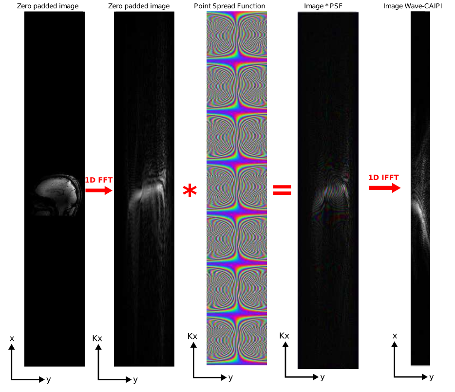
The different steps of the Wave-CAIPI strategy were simulated in MATLAB using a 3D phantom and an in-vivo brain scan (3D gradient-echo whole-brain 1 mm isotropic). We obtained the coil sensitivity maps from a single slice projection scan and computed the Point Spread Function. The under-sampled wave-image (Figure 1) was obtained by using the Wave equation (Equation 1) and by retrospectively under-sampling data. An iterative SENSE-reconstruction was used to reconstruct this image.
$$wave[x,y,z] = F_x^{-1} Psf[x,y,z](F_x C m[x,y,z]) \tag{1}$$
In the simulations, different combinations of Wave-CAIPI parameters were used for image generation and reconstruction. The following Wave-CAIPI parameters were simulated: Gy ,Gz ,Sinsy ,Sinsz and Pixel BW, which can be found in the Range of Spread function (Equation 2)[4].
$$R_g = \frac{2max(F_{inst})}{p_{bw}} + N_x \quad \quad \quad \quad F_{inst} = -γ (G_y cos(ω_y t) y + G_z sin(ω_z t) z) \tag{2}$$
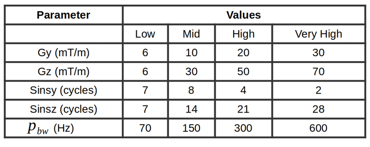
These parameters were further grouped into four categories (Table 1) for the simulations. The optimal parameter combination was found through three different analyses: the relation between the range-of-spread of the different grouped categories and the image quality; the effect of the number of cycles; and the effect of varying the Pixel BW. To characterize the image quality, three different metrics were calculated for each reconstruction: average G-factor, maximum G-factor and Root Mean Squared Error, which gave an indication of the noise amplification and error in the final image, respectively.

To investigate whether the gradient insert would be beneficial to the Wave-CAIPI method we compared simulations with the Wave-CAIPI parameters using the performance of the conventional gradient systems to simulations using the high efficiency gradient insert. This was done to find out if the same range-of-spread can be accomplished in a shorter period of time and if the insert coil’s ability of applying higher gradient amplitudes and number of cycles allows for a higher under-sampling factor without compromising image quality.

Results and Discussion

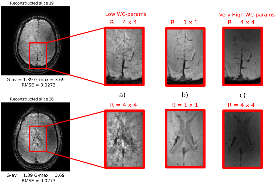
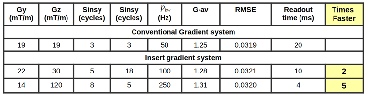
In Figure 2 we can see that less noise and residual aliasing artifacts are visible in the reconstruction using a Very High parameter configuration when compared to the Low parameter configuration. The reduction in artifacts comes from the larger range-of-spread that can be generated using the high performance of the insert gradient. The higher attainable gradient amplitude increases the maximum instantaneous frequency (increasing range-of-spread) which compensates for an increase in pixel bandwidth (reducing range-of-spread).

Table 2 shows that the readout time can be reduced up to 5-fold with only minor increases in average g-factor and RMSE. Here, the high slew rate of the gradient insert allows us to maintain sine-cycles while the high gradient amplitude of 120 mT/m ensures a large range of spread which both beneficially influence the reconstruction. Furthermore, the reduction in readout time might open up a pathway to combine Wave-CAIPI with an EPI readout. Such a combination is challenging using conventional gradients due to the trade-off between range-of-spread and pixel bandwidth.

In this work, we only look at the effect of applying a single-axis gradient insert to Wave-CAIPI. However, the simulation framework can be extended to multiple axes for which we foresee even larger acceleration potential when combined with Wave-CAIPI.

Conclusion

We have shown that the high performance of an insert gradient coil can be highly beneficial to improve Wave-CAIPI reconstructions. In simulations, this gradient insert combined with optimal Wave-CAIPI parameters would allow for 16-fold under-sampling (Ry x Rz = 4 x 4) whilst keeping similar image quality as a fully sampled readout using a conventional gradient setup. Moreover, the gradient insert could also shorten the readout time up to a factor of five, which could be useful for applying Wave-CAIPI in EPI sequences.

Acknowledgements

No acknowledgement found.