Introduction

Loud acoustic noise from gradient intensive sequences can cause anxiety in patients and lead to a degradation in image quality [1,2]. Therefore, sound level reduction is important to enhance patient comfort and ensure consistent image quality. This sound level reduction is usually achieved by reducing the amount of gradient switching. For example, methods like PETRA, RUFIS, ZTE BURST and Looping Star utilize a modified zero echo time acquisition and slowly updating gradients [3–6]. Alternatively, we have shown that considerable reduction in noise perception can be achieved by increasing the gradient switching frequency beyond the hearing threshold [7]. Here the readout gradient axis is switched at the inaudible frequency of 20 kHz. In this work, we have implemented fast and quiet anatomical brain imaging using this silent MRI readout setup (at 7T) for a 3D MPRAGE T₁-weighted sequence.

Methods

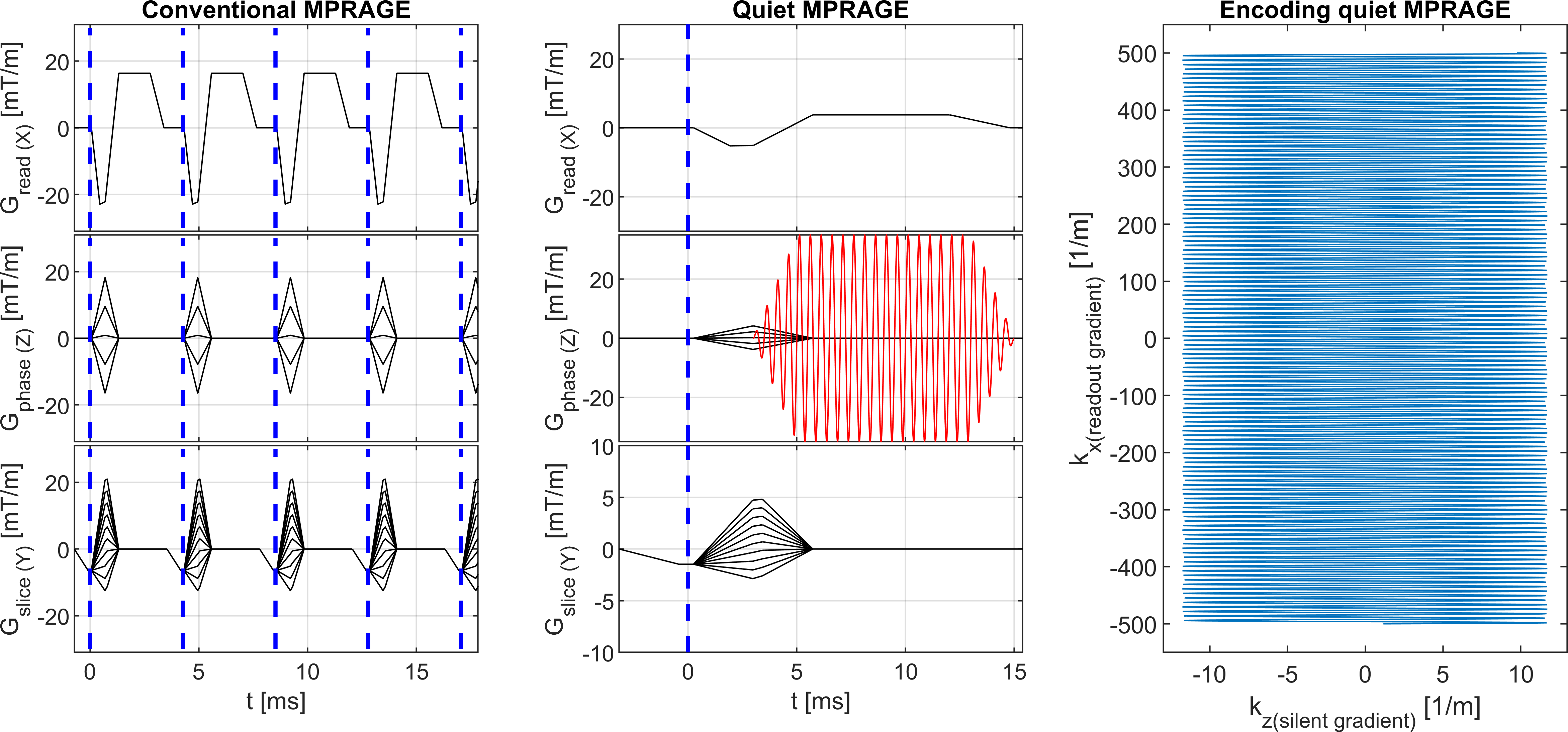
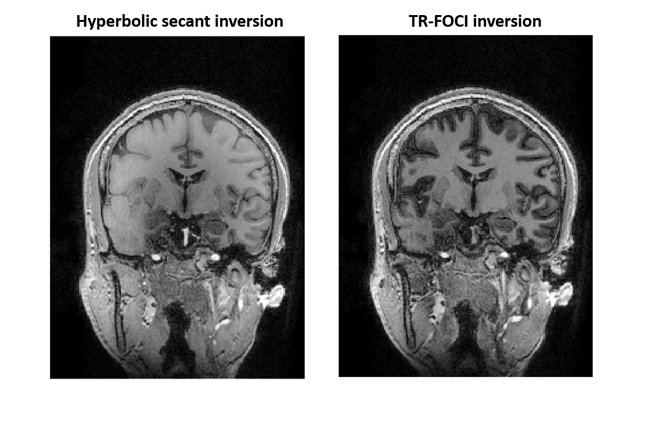
The silent gradient axis operates as an additional 4th gradient axis (z-direction) to the whole-body gradient system and consists of a lightweight gradient head insert driven by an audio amplifier (18 kW, Powersoft, Italy). This produces 28.6 mT/m at 20.2 kHz (3600T/m/s, and no noticeable PNS [8]). The setup features an integrated birdcage transmit coil, fits a 32-channel receive coil (NOVA Medical, USA), and was placed in a 7T MR system (Philips, The Netherlands).

The silent readout module uses an inaudible oscillating readout gradient in the phase-encoding direction to provide additional spatial encoding during the fast gradient-echo readout of the MPRAGE sequence (Figure 1). Due to the increased encoding efficiency, the sound production of the other, whole body, gradients in the sequence were decreased by reducing the slew rate without effecting the scan time. However, the lower slew rate did result in a longer minimum echo (TE) and repetition time (TR). To compensate for the longer TE and TR, the signal in white matter, gray matter and CSF was simulated using extended phase-graphs simulations, which allowed us to optimize the gray versus white matter contrast while nulling CSF in the quiet MPRAGE scan. Additionally, a TR-FOCI pulse was used for inversion to mitigate low B­₁⁺ amplitude and inhomogeneities and more uniform image contrast (Figure 2) [9]. A CAIPI-like sampling pattern was used to limit noise enhancements from variations in the sampling density.

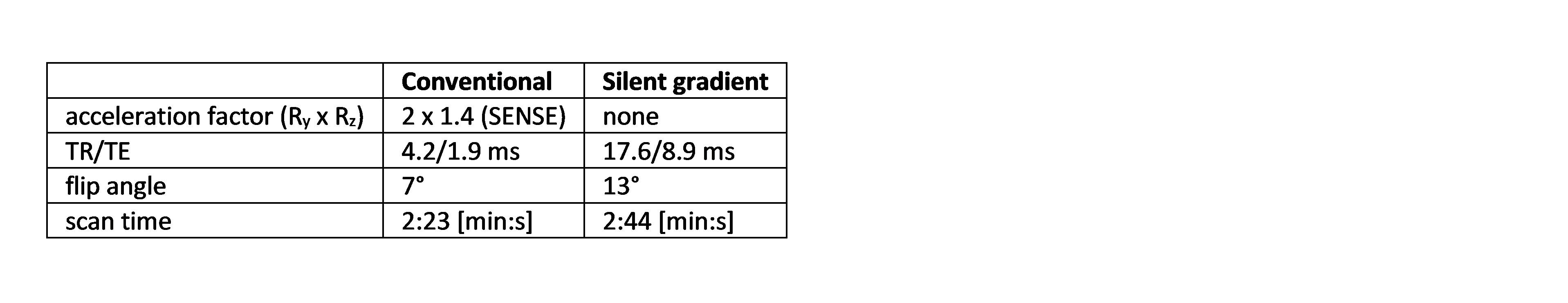
A volunteer was imaged using both the quiet and a conventional MPRAGE scan while positioned in the gradient insert. A whole-brain field-of-view of 256x256x172 mm³ was acquired with a 1 mm isotropic resolution, a shot interval of 3000 ms, radial (k_y-k_z) ordering, and an inversion time of 1000 ms (Table 1). Data was reconstructed offline in MATLAB using an iterative SENSE reconstruction [10,11]. For this reconstruction, the spatiotemporal behavior of the oscillating gradient field was first characterized using a field camera (Skope, Switzerland) and was used as an input for the reconstruction.

Relative sound measurements of both scans were performed using a condenser microphone (Behringer ECM8000). The audio data was processed in MATLAB. Here, exponential filtering and A-weighting was applied to mimic the fast response setting and output of a sound level meter. The same data was also used to determine the effect of the 20 kHz sound, which was estimated from Z-weighting of the audio signal.

Results and Discussion

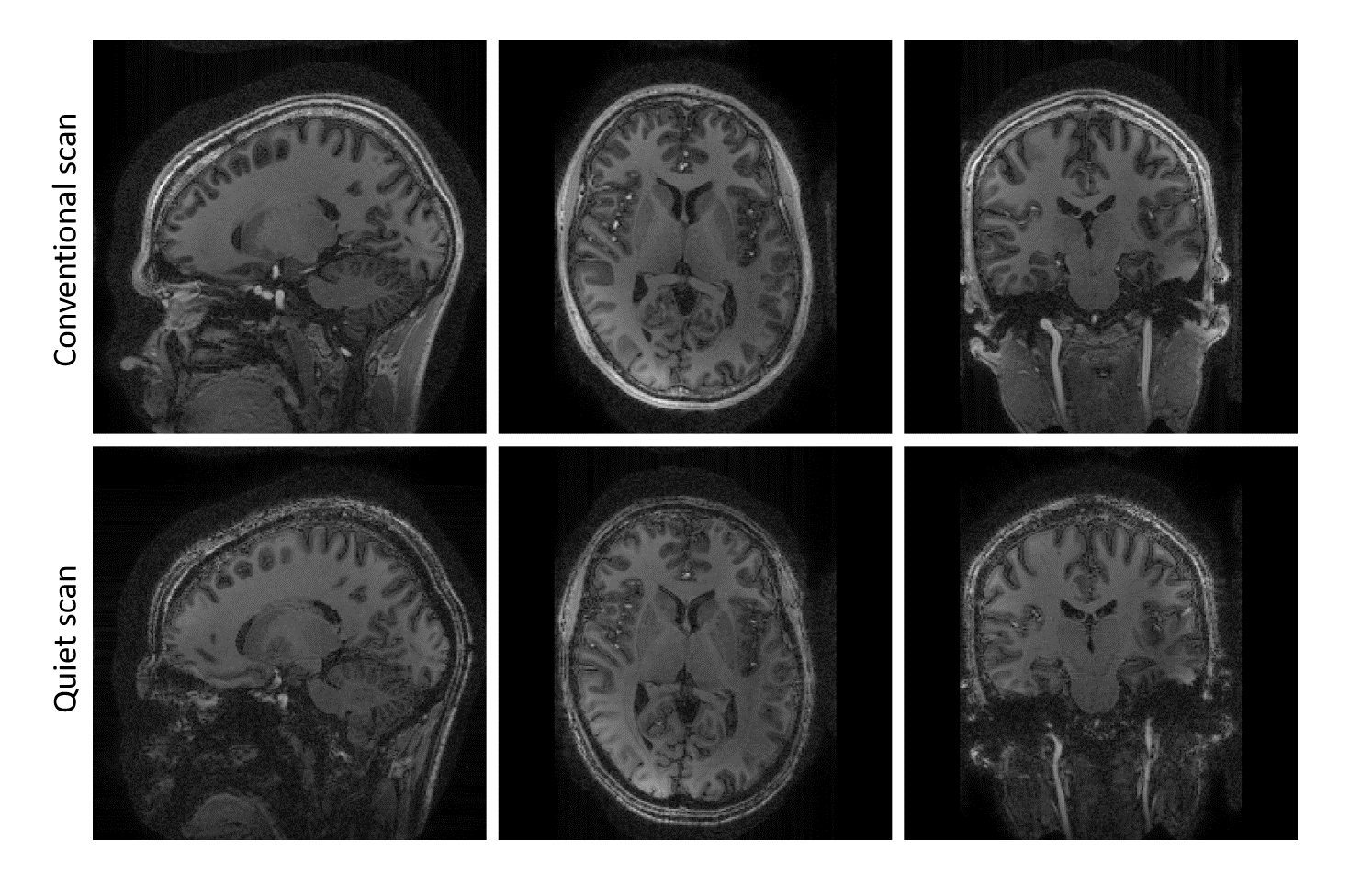
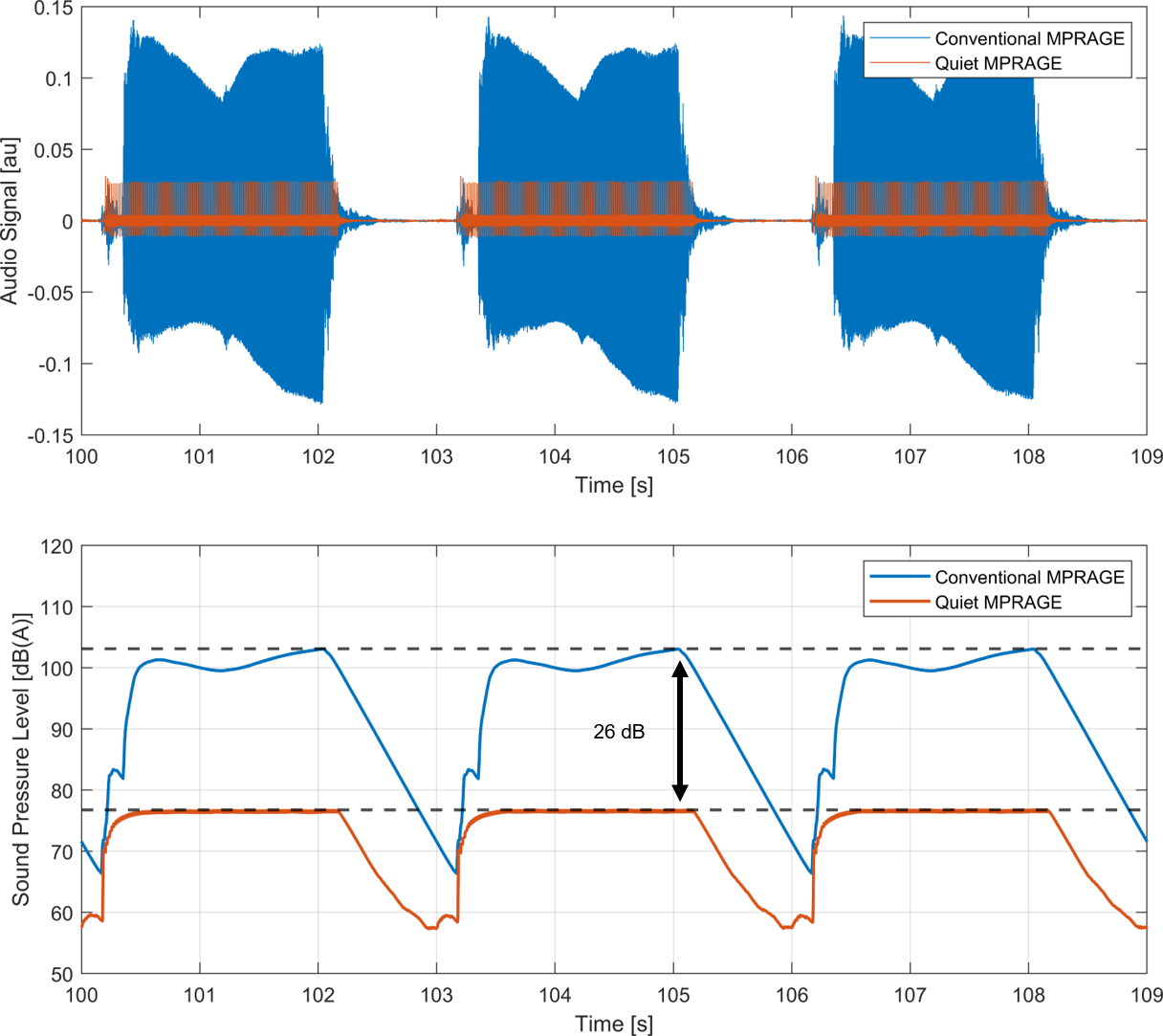
Figure 3 shows very similar gray and white matter contrast for both the conventional and quiet MPRAGE scans, which was expected from the EPG-simulations. Some residual loss of contrast is visible in both scans due to insufficiently low B­₁⁺ amplitude. Additionally, the quiet scan shows some signal loss in the neck region, which originates from the short linear region of the gradient insert. We foresee that part of the signal loss can be recovered by incorporating the non-linear field into the reconstruction using e.g. a PSF-reconstruction as is used in WAVE-CAIPI [12] or an expanded signal model [13].

Importantly, the sound measurements (Figure 4) show a 26 dB reduction in the peak sound pressure level during the scan. Here, the main source of residual sound originated from the slowly switching whole-body gradients resulting in a low-frequency humming sound during the MPRAGE readout. While not perceived as sound, the silent gradient axis nevertheless produces sound pressure. When this 20 kHz sound is included this still result in a 13 dB lower sound pressure level in the quiet scan compared to a traditional MPRAGE scan.

The quiet MPRAGE scan was 15% slower than the conventional scan due to duty cycle limitations of the current audio amplifier, which limited the gradient amplitude. However, the silent gradient axis still allows for an additional acceleration by using traditional parallel imaging techniques in the slice-encoding direction, which would allow us to compensate for the hardware limitations.

Conclusion

We have shown that a silent gradient axis can considerably reduce sound (26 dB) for MPRAGE scans while maintaining similar image contrast as a conventional MPRAGE scan. Such a silent gradient axis provides a way to fast and quiet imaging that can be readily translated to 3 tesla field strengths with the potential to greatly improve patient comfort for a wide variety of clinical scans.

Acknowledgements

No acknowledgement found.