Introduction

Prostate cancer is one of the most commonly diagnosed cancers, however with early screening and timely treatment, the survival rate of patients has been improved significantly. Radiotherapy treatment planning is conventionally performed through CT scanning, however, repeated CT scans increase radiation exposure. This motivates many studies on MR-only radiotherapy planning, which attempts to derive electron density information of CT from MR images. Recent studies^1,2 have shown that deep learning can generate synthetic CT images (sCT) with good dosimetry comparable to real CT acquisition. Contouring or delineation of the prostate and surrounding tissues to inspect radiation dose distribution is also an important step that requires precious time and manual labor. In this study, we propose CycleSeg, a network that can perform sCT generation and organ segmentation from an input T2-weighted MR image to streamline the treatment process.

Method

Data acquisition and processing
We utilized 115 sets of simulation CT scans of patients with prostate cancer who underwent radiotherapy with or without surgery between January 2016 and July 2018 at our medical center. The simulation CT scans were performed with GE Healthcare Discovery CT590 RT. The field of view (FOV) was 50cm, the slice-thickness between the consecutive axial CT images was 2.5 mm, and the matrix size and resolution were 512×512 and 0.98×0.98 mm². Contours of organs-of-interest (prostate, left and right femur head, bladder, rectum, and penile bulb) were manually annotated on the CT data.
MRI scans were conducted immediately after the simulation CT scans with a Philips 3.0 T Ingenia MR. T2 weighted MR images were obtained with FOV = 400×400×200mm³, matrix size = 960×960, TR/TE = 6152 ms/100 ms.
The data were manually inspected to remove those with unusual artifacts, resulting in 96 pairs of MRI/CT volumes. To process the data for training the networks, we first resampled both MRI and CT volumes to a common 1.3×1.3×2.5mm³ spacing and register the MRI volume to CT volume with affine transformation in simpleITK^3-5. We cropped the central 384×384 in the axial plane to remove the background. To perform intensity normalization, we clipped Hounsfield units (HU) of CT data to [-200, 1300] range, which was linearly mapped to [-1, 1] range. For the MRI data, we normalized the intensity by subtracting the mean and dividing by 2.5 times the standard deviation of the voxels inside the body and clipped the normalized values to [-1,1] range.

Network architecture and training:
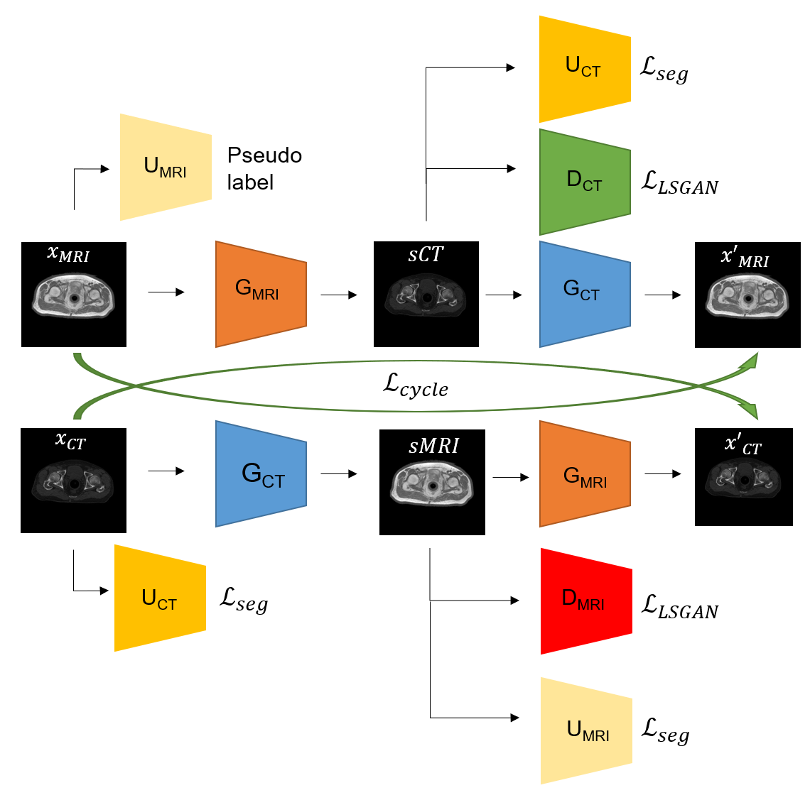
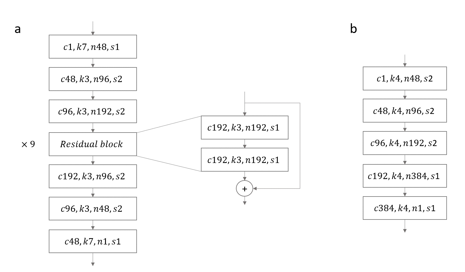
CycleSeg consists of a CycleGAN⁶ and 2 UNets⁷, whose structures are shown in Figures 1 and 2. Similar to (8), CycleSeg enforces shape consistency to improve the segmentation and synthesis results. Since only the CT segmentation is available, we proposed to use pseudo-label created from the MRI images by the UNet-MRI to train the UNet-CT with sCT images. The following loss is minimized during the training process:
$$L(x_{MRI},x_{CT}) = L_{LSGAN} + \lambda_{cycle} L_{cycle} + \lambda_{idt} L_{idt} + \lambda_{ref} L_{ref} + \lambda_{seg} L_{seg} (1)$$
$$$L_{LSGAN}$$$: least squared GAN loss⁹
$$$L_{cycle}$$$: cyclic loss between reconstructed ($$$x'_{MRI}, x'_{CT}$$$) and original image ($$$x_{MRI}, x_{CT}$$$)
$$$L_{idt}$$$: identity loss of transforming image from one domain with the same corresponding generator ( $$$G_{MRI}$$$ should not modify $$$x_{CT}$$$)
$$$L_{ref}$$$ : pixel-wise loss between anatomically close pairs of synthetic CT/MRI and real CT/MRI
$$$L_{seg}$$$: cross-entropy loss with real CT label and pseudo-label from $$$U_{MRI}(x_{MRI})$$$
$$$\lambda_{cycle},\lambda_{idt},\lambda_{ref},\lambda_{seg}$$$ : hyperparameters that control the contribution from each loss term. These are set as 10, 5, 10, 1 respectively.
Four models were trained with different losses to verify the effectiveness of the approach.
Model 1: CycleGAN with Eq. (1) loss (proposed "CycleSeg")
Model 2: CycleGAN, trained without $$$L_{ref}$$$ and $$$L_{seg}$$$
Model 3: CycleGAN with $$$L_{ref}$$$
Model 4: CycleGAN with $$$L_{ref}$$$ and segmentation reference loss $$$L_{ref, seg}$$$ (using CT segmentation label of CT slice anatomically close to MRI slice as sCT segmentation label).
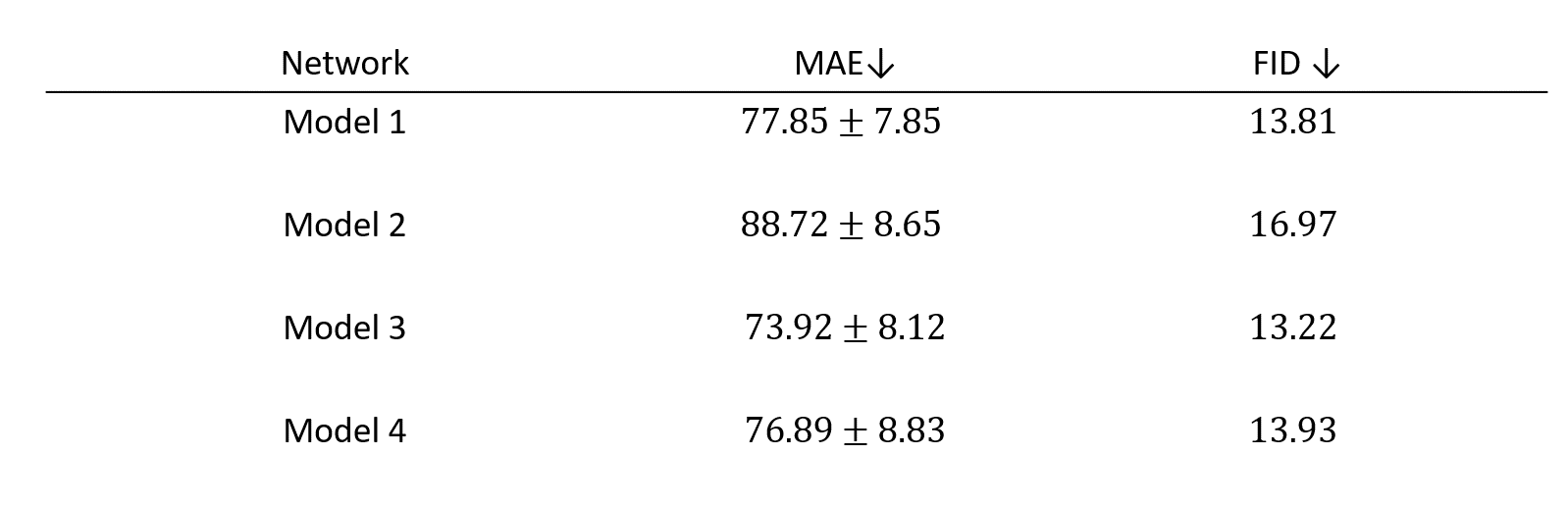
We calculated mean absolute error (MAE) of HU between the closely matched slices of real and synthetic CT. We also used Frechet inception distance (FID)¹⁰ as it is more indicative of visual quality.

Result

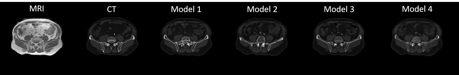
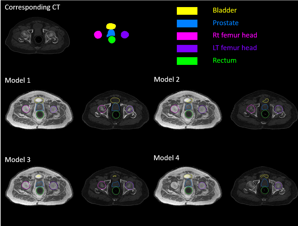
Table 1 shows the quantitative result on the test set of the four networks. The addition of reference loss improves the MAE and FID while the inclusion of segmentation network does not seem to improve the synthesis result. Figure 3 showed the qualitative comparison of a representative sCT from the four networks. Addition of the reference loss improves the appearance of the bones while segmentation loss does not seem to provide any visible benefit. Figure 4 showed the qualitative comparison of the segmentation performance for a representative slice and the effectiveness of Model 1 that uses Eq (1) as the loss function. Model 1 showed good segmentation results for all organs when compared to the segmentation of the matched CT slice. The other three models failed to successfully segment the bladder. Notably, Model 4 that was trained with the reference segmentation loss appeared to perform worse compared to the pseudo label loss of Model 1, possibly due to registration mismatch for Model 4.

Conclusion

By the addition of reference and segmentation losses, CycleSeg (Model 1) provides both high quality sCT synthesis and organ segmentation (contour) in prostate area, which can be beneficial for MR-only prostate cancer radiotherapy planning.

Acknowledgements

No acknowledgement found.